Infinite matter, from the electron gas to nuclear matter
Morten Hjorth-Jensen, National Superconducting Cyclotron Laboratory and Department of Physics and Astronomy, Michigan State University, East Lansing, MI 48824, USA & Department of Physics, University of Oslo, Oslo, Norway
July 2015
Table of contents
Introduction to studies of infinite matter
The infinite electron gas
The infinite electron gas as a homogenous system
Periodic boundary conditions
Defining the Hamiltonian operator
Single-particle Hartree-Fock energy
Exercise 1: Hartree-Fock single-particle solution for the electron gas
Exercise 2: Hartree-Fock ground state energy for the electron gas in three dimensions
Preparing the ground for numerical calculations; kinetic energy and Ewald term
Ewald correction term
Interaction in momentum space
Antisymmetrized matrix elements in three dimensions
Periodic boundary conditions and single-particle states
Magic numbers for the two-dimensional electron gas
Hartree-Fock energies
Exercise 3: Magic numbers for the three-dimensional electron gas and perturbation theory to second order
Infinite nuclear matter and neutron star matter
Brueckner-Hartree-Fock theory
Exercise 4: Magic numbers for infinite matter and the Minnesota interaction model
Introduction to studies of infinite matter
Studies of infinite nuclear matter play an important role in nuclear physics. The aim of this part of the lectures is to provide the necessary ingredients for perfoming studies of neutron star matter (or matter in \( \beta \)-equilibrium) and symmetric nuclear matter. We start however with the electron gas in two and three dimensions for both historical and pedagogical reasons. Since there are several benchmark calculations for the electron gas, this small detour will allow us to establish the necessary formalism. Thereafter we will study infinite nuclear matter
- at the Hartree-Fock with realistic nuclear forces and
- using many-body methods like coupled-cluster theory or in-medium SRG as discussed in our previous sections.
The infinite electron gas
The electron gas is perhaps the only realistic model of a
system of many interacting particles that allows for a solution
of the Hartree-Fock equations on a closed form. Furthermore, to first order in the interaction, one can also
compute on a closed form the total energy and several other properties of a many-particle systems.
The model gives a very good approximation to the properties of valence electrons in metals.
The assumptions are
- System of electrons that is not influenced by external forces except by an attraction provided by a uniform background of ions. These ions give rise to a uniform background charge. The ions are stationary.
- The system as a whole is neutral.
- We assume we have \( N_e \) electrons in a cubic box of length \( L \) and volume \( \Omega=L^3 \). This volume contains also a uniform distribution of positive charge with density \( N_ee/\Omega \).
The homogeneous electron gas is one of the few examples of a system of many
interacting particles that allows for a solution of the mean-field
Hartree-Fock equations on a closed form. To first order in the
electron-electron interaction, this applies to ground state properties
like the energy and its pertinent equation of state as well. The
homogeneus electron gas is a system of electrons that is not
influenced by external forces except by an attraction provided by a
uniform background of ions. These ions give rise to a uniform
background charge. The ions are stationary and the system as a whole
is neutral.
Irrespective of this simplicity, this system, in both two and
three-dimensions, has eluded a proper description of correlations in
terms of various first principle methods, except perhaps for quantum
Monte Carlo methods. In particular, the diffusion Monte Carlo
calculations of Ceperley
and Ceperley and Tanatar
are presently still considered as the
best possible benchmarks for the two- and three-dimensional electron
gas.
The electron gas, in
two or three dimensions is thus interesting as a test-bed for
electron-electron correlations. The three-dimensional
electron gas is particularly important as a cornerstone
of the local-density approximation in density-functional
theory. In the physical world, systems
similar to the three-dimensional electron gas can be
found in, for example, alkali metals and doped
semiconductors. Two-dimensional electron fluids are
observed on metal and liquid-helium surfaces, as well as
at metal-oxide-semiconductor interfaces. However, the Coulomb
interaction has an infinite range, and therefore
long-range correlations play an essential role in the
electron gas.
At low densities, the electrons become
localized and form a lattice. This so-called Wigner
crystallization is a direct consequence
of the long-ranged repulsive interaction. At higher
densities, the electron gas is better described as a
liquid.
When using, for example, Monte Carlo methods the electron gas must be approximated
by a finite system. The long-range Coulomb interaction
in the electron gas causes additional finite-size effects that are not
present in other infinite systems like nuclear matter or neutron star matter.
This poses additional challenges to many-body methods when applied
to the electron gas.
The infinite electron gas as a homogenous system
This is a homogeneous system and the one-particle wave functions are given by plane wave functions normalized to a volume \( \Omega \)
for a box with length \( L \) (the limit \( L\rightarrow \infty \) is to be taken after we have computed various expectation values)
$$
\psi_{\mathbf{k}\sigma}(\mathbf{r})= \frac{1}{\sqrt{\Omega}}\exp{(i\mathbf{kr})}\xi_{\sigma}
$$
where \( \mathbf{k} \) is the wave number and \( \xi_{\sigma} \) is a spin function for either spin up or down
$$
\xi_{\sigma=+1/2}=\left(\begin{array}{c} 1 \\ 0 \end{array}\right) \hspace{0.5cm}
\xi_{\sigma=-1/2}=\left(\begin{array}{c} 0 \\ 1 \end{array}\right).
$$
Periodic boundary conditions
We assume that we have periodic boundary conditions which limit the allowed wave numbers to
$$
k_i=\frac{2\pi n_i}{L}\hspace{0.5cm} i=x,y,z \hspace{0.5cm} n_i=0,\pm 1,\pm 2, \dots
$$
We assume first that the electrons interact via a central, symmetric and translationally invariant
interaction \( V(r_{12}) \) with
\( r_{12}=|\mathbf{r}_1-\mathbf{r}_2| \). The interaction is spin independent.
The total Hamiltonian consists then of kinetic and potential energy
$$
\hat{H} = \hat{T}+\hat{V}.
$$
The operator for the kinetic energy can be written as
$$
\hat{T}=\sum_{\mathbf{k}\sigma}\frac{\hbar^2k^2}{2m}a_{\mathbf{k}\sigma}^{\dagger}a_{\mathbf{k}\sigma}.
$$
Defining the Hamiltonian operator
The Hamiltonian operator is given by
$$
\hat{H}=\hat{H}_{el}+\hat{H}_{b}+\hat{H}_{el-b},
$$
with the electronic part
$$
\hat{H}_{el}=\sum_{i=1}^N\frac{p_i^2}{2m}+\frac{e^2}{2}\sum_{i\ne j}\frac{e^{-\mu |\mathbf{r}_i-\mathbf{r}_j|}}{|\mathbf{r}_i-\mathbf{r}_j|},
$$
where we have introduced an explicit convergence factor
(the limit \( \mu\rightarrow 0 \) is performed after having calculated the various integrals).
Correspondingly, we have
$$
\hat{H}_{b}=\frac{e^2}{2}\int\int d\mathbf{r}d\mathbf{r}'\frac{n(\mathbf{r})n(\mathbf{r}')e^{-\mu |\mathbf{r}-\mathbf{r}'|}}{|\mathbf{r}-\mathbf{r}'|},
$$
which is the energy contribution from the positive background charge with density
\( n(\mathbf{r})=N/\Omega \). Finally,
$$
\hat{H}_{el-b}=-\frac{e^2}{2}\sum_{i=1}^N\int d\mathbf{r}\frac{n(\mathbf{r})e^{-\mu |\mathbf{r}-\mathbf{x}_i|}}{|\mathbf{r}-\mathbf{x}_i|},
$$
is the interaction between the electrons and the positive background.
Single-particle Hartree-Fock energy
In the first exercise below we show that the Hartree-Fock energy can be written as
$$
\varepsilon_{k}^{HF}=\frac{\hbar^{2}k^{2}}{2m_e}-\frac{e^{2}}
{\Omega^{2}}\sum_{k'\leq
k_{F}}\int d\mathbf{r}e^{i(\mathbf{k}'-\mathbf{k})\mathbf{r}}\int
d\mathbf{r'}\frac{e^{i(\mathbf{k}-\mathbf{k}')\mathbf{r}'}}
{\vert\mathbf{r}-\mathbf{r}'\vert}
$$
resulting in
$$
\varepsilon_{k}^{HF}=\frac{\hbar^{2}k^{2}}{2m_e}-\frac{e^{2}
k_{F}}{2\pi}
\left[
2+\frac{k_{F}^{2}-k^{2}}{kk_{F}}ln\left\vert\frac{k+k_{F}}
{k-k_{F}}\right\vert
\right]
$$
The previous result can be rewritten in terms of the density
$$
n= \frac{k_F^3}{3\pi^2}=\frac{3}{4\pi r_s^3},
$$
where \( n=N_e/\Omega \), \( N_e \) being the number of electrons, and \( r_s \) is the radius of a sphere which represents the volum per conducting electron.
It can be convenient to use the Bohr radius \( a_0=\hbar^2/e^2m_e \).
For most metals we have a relation \( r_s/a_0\sim 2-6 \). The quantity \( r_s \) is dimensionless.
In the second exercise below we find that
the total energy
\( E_0/N_e=\langle\Phi_{0}|\hat{H}|\Phi_{0}\rangle/N_e \) for
for this system to first order in the interaction is given as
$$
E_0/N_e=\frac{e^2}{2a_0}\left[\frac{2.21}{r_s^2}-\frac{0.916}{r_s}\right].
$$
Exercise 1: Hartree-Fock single-particle solution for the electron gas
The electron gas model allows closed form solutions for quantities like the
single-particle Hartree-Fock energy. The latter quantity is given by the following expression
$$
\varepsilon_{k}^{HF}=\frac{\hbar^{2}k^{2}}{2m}-\frac{e^{2}}
{V^{2}}\sum_{k'\leq
k_{F}}\int d\mathbf{r}e^{i(\mathbf{k'}-\mathbf{k})\mathbf{r}}\int
d\mathbf{r}'\frac{e^{i(\mathbf{k}-\mathbf{k'})\mathbf{r}'}}
{\vert\mathbf{r}-\mathbf{r'}\vert}
$$
a)
Show first that
$$
\varepsilon_{k}^{HF}=\frac{\hbar^{2}k^{2}}{2m}-\frac{e^{2}
k_{F}}{2\pi}
\left[
2+\frac{k_{F}^{2}-k^{2}}{kk_{F}}ln\left\vert\frac{k+k_{F}}
{k-k_{F}}\right\vert
\right]
$$
Hint.
Hint: Introduce the convergence factor
\( e^{-\mu\vert\mathbf{r}-\mathbf{r}'\vert} \)
in the potential and use \( \sum_{\mathbf{k}}\rightarrow
\frac{V}{(2\pi)^{3}}\int d\mathbf{k} \)
Solution.
We want to show that, given the Hartree-Fock equation for the electron gas
$$
\varepsilon_{k}^{HF}=\frac{\hbar^{2}k^{2}}{2m}-\frac{e^{2}}
{V^{2}}\sum_{p\leq
k_{F}}\int d\mathbf{r}\exp{(i(\mathbf{p}-\mathbf{k})\mathbf{r})}\int
d\mathbf{r}'\frac{\exp{(i(\mathbf{k}-\mathbf{p})\mathbf{r}'})}
{\vert\mathbf{r}-\mathbf{r'}\vert}
$$
the single-particle energy can be written as
$$
\varepsilon_{k}^{HF}=\frac{\hbar^{2}k^{2}}{2m}-\frac{e^{2}
k_{F}}{2\pi}
\left[
2+\frac{k_{F}^{2}-k^{2}}{kk_{F}}ln\left\vert\frac{k+k_{F}}
{k-k_{F}}\right\vert
\right].
$$
We introduce the convergence factor
\( e^{-\mu\vert\mathbf{r}-\mathbf{r}'\vert} \)
in the potential and use \( \sum_{\mathbf{k}}\rightarrow
\frac{V}{(2\pi)^{3}}\int d\mathbf{k} \). We can then rewrite the integral as
$$
\begin{align}
\frac{e^{2}}
{V^{2}}\sum_{k'\leq
k_{F}}\int d\mathbf{r}\exp{(i(\mathbf{k'}-\mathbf{k})\mathbf{r})}\int
d\mathbf{r}'\frac{\exp{(i(\mathbf{k}-\mathbf{p})\mathbf{r}'})}
{\vert\mathbf{r}-\mathbf{r'}\vert}= & \\
\frac{e^{2}}{V (2\pi)^3} \int d\mathbf{r}\int
\frac{d\mathbf{r}'}{\vert\mathbf{r}-\mathbf{r'}\vert}\exp{(-i\mathbf{k}(\mathbf{r}-\mathbf{r}'))}\int d\mathbf{p}\exp{(i\mathbf{p}(\mathbf{r}-\mathbf{r}'))},
\end{align}
$$
and introducing the abovementioned convergence factor we have
$$
\begin{align}
\lim_{\mu \to 0}\frac{e^{2}}{V (2\pi)^3} \int d\mathbf{r}\int d\mathbf{r}'\frac{\exp{(-\mu\vert\mathbf{r}-\mathbf{r}'\vert})}{\vert\mathbf{r}-\mathbf{r'}\vert}\int d\mathbf{p}\exp{(i(\mathbf{p}-\mathbf{k})(\mathbf{r}-\mathbf{r}'))}.
\end{align}
$$
With a change variables to \( \mathbf{x} = \mathbf{r}-\mathbf{r}' \) and \( \mathbf{y}=\mathbf{r}' \) we rewrite the last integral as
$$
\lim_{\mu \to 0}\frac{e^{2}}{V (2\pi)^3} \int d\mathbf{p}\int d\mathbf{y}\int d\mathbf{x}\exp{(i(\mathbf{p}-\mathbf{k})\mathbf{x})}\frac{\exp{(-\mu\vert\mathbf{x}\vert})}{\vert\mathbf{x}\vert}.
$$
The integration over \( \mathbf{x} \) can be performed using spherical coordinates, resulting in (with \( x=\vert \mathbf{x}\vert \))
$$
\int d\mathbf{x}\exp{(i(\mathbf{p}-\mathbf{k})\mathbf{x})}\frac{\exp{(-\mu\vert\mathbf{x}\vert})}{\vert\mathbf{x}\vert}=\int x^2 dx d\phi d\cos{(\theta)}\exp{(i(\mathbf{p}-\mathbf{k})x\cos{(\theta))}}\frac{\exp{(-\mu x)}}{x}.
$$
We obtain
$$
\begin{align}
4\pi \int dx \frac{ \sin{(\vert \mathbf{p}-\mathbf{k}\vert)x} }{\vert \mathbf{p}-\mathbf{k}\vert}{\exp{(-\mu x)}}= \frac{4\pi}{\mu^2+\vert \mathbf{p}-\mathbf{k}\vert^2}.
\end{align}
$$
This results gives us
$$
\begin{align}
\lim_{\mu \to 0}\frac{e^{2}}{V (2\pi)^3} \int d\mathbf{p}\int d\mathbf{y}\frac{4\pi}{\mu^2+\vert \mathbf{p}-\mathbf{k}\vert^2}=\lim_{\mu \to 0}\frac{e^{2}}{ 2\pi^2} \int d\mathbf{p}\frac{1}{\mu^2+\vert \mathbf{p}-\mathbf{k}\vert^2},
\end{align}
$$
where we have used that the integrand on the left-hand side does not depend on \( \mathbf{y} \) and that \( \int d\mathbf{y}=V \).
Introducing spherical coordinates we can rewrite the integral as
$$
\begin{align}
\lim_{\mu \to 0}\frac{e^{2}}{ 2\pi^2} \int d\mathbf{p}\frac{1}{\mu^2+\vert \mathbf{p}-\mathbf{k}\vert^2}=\frac{e^{2}}{ 2\pi^2} \int d\mathbf{p}\frac{1}{\vert \mathbf{p}-\mathbf{k}\vert^2}=& \\
\frac{e^{2}}{\pi} \int_0^{k_F} p^2dp\int_0^{\pi} d\theta\cos{(\theta)}\frac{1}{p^2+k^2-2pk\cos{(\theta)}},
\end{align}
$$
and with the change of variables \( \cos{(\theta)}=u \) we have
$$
\frac{e^{2}}{\pi} \int_0^{k_F} p^2dp\int_{0}^{\pi} d\theta\cos{(\theta)}\frac{1}{p^2+k^2-2pk\cos{(\theta)}}=\frac{e^{2}}{\pi} \int_0^{k_F} p^2dp\int_{-1}^{1} du\frac{1}{p^2+k^2-2pku},
$$
which gives
$$
\frac{e^{2}}{k\pi} \int_0^{k_F} pdp\left\{ln(\vert p+k\vert)-ln(\vert p-k\vert)\right\}.
$$
Introducing new variables \( x=p+k \) and \( y=p-k \), we obtain after some straightforward reordering of the integral
$$
\frac{e^{2}}{k\pi}\left[
kk_F+\frac{k_{F}^{2}-k^{2}}{kk_{F}}ln\left\vert\frac{k+k_{F}}
{k-k_{F}}\right\vert
\right],
$$
which gives the abovementioned expression for the single-particle energy.
b)
Rewrite the above result as a function of the density
$$
n= \frac{k_F^3}{3\pi^2}=\frac{3}{4\pi r_s^3},
$$
where \( n=N/V \), \( N \) being the number of particles, and \( r_s \) is the radius of a sphere which represents the volum per conducting electron.
Solution.
Introducing the dimensionless quantity \( x=k/k_F \) and the function
$$
F(x) = \frac{1}{2}+\frac{1-x^2}{4x}\ln{\left\vert \frac{1+x}{1-x}\right\vert},
$$
we can rewrite the single-particle Hartree-Fock energy as
$$
\varepsilon_{k}^{HF}=\frac{\hbar^{2}k^{2}}{2m}-\frac{2e^{2}
k_{F}}{\pi}F(k/k_F),
$$
and dividing by the non-interacting contribution at the Fermi level,
$$
\varepsilon_{0}^{F}=\frac{\hbar^{2}k_F^{2}}{2m},
$$
we have
$$
\frac{\varepsilon_{k}^{HF} }{\varepsilon_{0}^{F}}=x^2-\frac{e^2m}{\hbar^2 k_F\pi}F(x)=x^2-\frac{4}{\pi k_Fa_0}F(x),
$$
where \( a_0=0.0529 \) nm is the Bohr radius, setting thereby a natural length scale.
By introducing the radius \( r_s \) of a sphere whose volume is the volume occupied by each electron, we can rewrite the previous equation in terms of \( r_s \) using that the electron density \( n=N/V \)
$$
n=\frac{k_F^3}{3\pi^2} = \frac{3}{4\pi r_s^3},
$$
we have (with \( k_F=1.92/r_s \),
$$
\frac{\varepsilon_{k}^{HF} }{\varepsilon_{0}^{F}}=x^2-\frac{e^2m}{\hbar^2 k_F\pi}F(x)=x^2-\frac{r_s}{a_0}0.663F(x),
$$
with \( r_s \sim 2-6 \) for most metals.
It can be convenient to use the Bohr radius \( a_0=\hbar^2/e^2m \).
For most metals we have a relation \( r_s/a_0\sim 2-6 \).
c)
Make a plot of the free electron energy and the Hartree-Fock energy and discuss the behavior around the Fermi surface. Extract also the Hartree-Fock band width \( \Delta\varepsilon^{HF} \) defined as
$$
\Delta\varepsilon^{HF}=\varepsilon_{k_{F}}^{HF}-
\varepsilon_{0}^{HF}.
$$
Compare this results with the corresponding one for a free electron and comment your results. How large is the contribution due to the exchange term in the Hartree-Fock equation?
Solution.
We can now define the so-called band gap, that is the scatter between the maximal and the minimal value of the electrons in the conductance band of a metal (up to the Fermi level).
For \( x=1 \) and \( r_s/a_0=4 \) we have
$$
\frac{\varepsilon_{k=k_F}^{HF} }{\varepsilon_{0}^{F}} = -0.326,
$$
and for \( x=0 \) we have
$$
\frac{\varepsilon_{k=0}^{HF} }{\varepsilon_{0}^{F}} = -2.652,
$$
which results in a gap at the Fermi level of
$$
\Delta \varepsilon^{HF} = \frac{\varepsilon_{k=k_F}^{HF} }{\varepsilon_{0}^{F}}-\frac{\varepsilon_{k=0}^{HF} }{\varepsilon_{0}^{F}} = 2.326.
$$
This quantity measures the deviation from the \( k=0 \) single-particle energy and the energy at the Fermi level.
The general result is
$$
\Delta \varepsilon^{HF} = 1+\frac{r_s}{a_0}0.663.
$$
The following python code produces a plot of the electron energy for a free electron (only kinetic energy) and
for the Hartree-Fock solution. We have chosen here a ratio \( r_s/a_0=4 \) and the equations are plotted as funtions
of \( k/f_F \).
import numpy as np
from math import log
from  matplotlib import pyplot as plt
from matplotlib import rc, rcParams
import matplotlib.units as units
import matplotlib.ticker as ticker
rc('text',usetex=True)
rc('font',**{'family':'serif','serif':['Hartree-Fock energy']})
font = {'family' : 'serif',
        'color'  : 'darkred',
        'weight' : 'normal',
        'size'   : 16,
        }

N = 100
x = np.linspace(0.0, 2.0,N)
F = 0.5+np.log(abs((1.0+x)/(1.0-x)))*(1.0-x*x)*0.25/x
y = x*x -4.0*0.663*F

plt.plot(x, y, 'b-')
plt.plot(x, x*x, 'r-')
plt.title(r'{\bf Hartree-Fock single-particle energy for electron gas}', fontsize=20)
plt.text(3, -40, r'Parameters: $r_s/a_0=4$', fontdict=font)
plt.xlabel(r'$k/k_F$',fontsize=20)
plt.ylabel(r'$\varepsilon_k^{HF}/\varepsilon_0^F$',fontsize=20)
# Tweak spacing to prevent clipping of ylabel
plt.subplots_adjust(left=0.15)
plt.savefig('hartreefockspelgas.pdf', format='pdf')
plt.show()
From the plot we notice that the exchange term increases considerably the band gap
compared with the non-interacting gas of electrons.
We will now define a quantity called the effective mass.
For \( \vert\mathbf{k}\vert \) near \( k_{F} \), we can Taylor expand the Hartree-Fock energy as
$$
\varepsilon_{k}^{HF}=\varepsilon_{k_{F}}^{HF}+
\left(\frac{\partial\varepsilon_{k}^{HF}}{\partial k}\right)_{k_{F}}(k-k_{F})+\dots
$$
If we compare the latter with the corresponding expressiyon for the non-interacting system
$$
\varepsilon_{k}^{(0)}=\frac{\hbar^{2}k^{2}_{F}}{2m}+
\frac{\hbar^{2}k_{F}}{m}\left(k-k_{F}\right)+\dots ,
$$
we can define the so-called effective Hartree-Fock mass as
$$
m_{HF}^{*}\equiv\hbar^{2}k_{F}\left(
\frac{\partial\varepsilon_{k}^{HF}}
{\partial k}\right)_{k_{F}}^{-1}
$$
d)
Compute \( m_{HF}^{*} \) and comment your results.
e)
Show that the level density (the number of single-electron states per unit energy) can be written as
$$
n(\varepsilon)=\frac{Vk^{2}}{2\pi^{2}}\left(
\frac{\partial\varepsilon}{\partial k}\right)^{-1}
$$
Calculate \( n(\varepsilon_{F}^{HF}) \) and comment the results.
Exercise 2: Hartree-Fock ground state energy for the electron gas in three dimensions
We consider a system of electrons in infinite matter, the so-called electron gas. This is a homogeneous system and the one-particle states are given by plane wave function normalized to a volume \( \Omega \)
for a box with length \( L \) (the limit \( L\rightarrow \infty \) is to be taken after we have computed various expectation values)
$$
\psi_{\mathbf{k}\sigma}(\mathbf{r})= \frac{1}{\sqrt{\Omega}}\exp{(i\mathbf{kr})}\xi_{\sigma}
$$
where \( \mathbf{k} \) is the wave number and \( \xi_{\sigma} \) is a spin function for either spin up or down
$$
\xi_{\sigma=+1/2}=\left(\begin{array}{c} 1 \\ 0 \end{array}\right) \hspace{0.5cm}
\xi_{\sigma=-1/2}=\left(\begin{array}{c} 0 \\ 1 \end{array}\right).
$$
We assume that we have periodic boundary conditions which limit the allowed wave numbers to
$$
k_i=\frac{2\pi n_i}{L}\hspace{0.5cm} i=x,y,z \hspace{0.5cm} n_i=0,\pm 1,\pm 2, \dots
$$
We assume first that the particles interact via a central, symmetric and translationally invariant
interaction \( V(r_{12}) \) with
\( r_{12}=|\mathbf{r}_1-\mathbf{r}_2| \). The interaction is spin independent.
The total Hamiltonian consists then of kinetic and potential energy
$$
\hat{H} = \hat{T}+\hat{V}.
$$
The operator for the kinetic energy is given by
$$
\hat{T}=\sum_{\mathbf{k}\sigma}\frac{\hbar^2k^2}{2m}a_{\mathbf{k}\sigma}^{\dagger}a_{\mathbf{k}\sigma}.
$$
a)
Find the expression for the interaction
\( \hat{V} \) expressed with creation and annihilation operators. The expression for the interaction
has to be written in \( k \) space, even though \( V \) depends only on the relative distance. It means that you need to set up the Fourier transform \( \langle \mathbf{k}_i\mathbf{k}_j| V | \mathbf{k}_m\mathbf{k}_n\rangle \).
Solution.
A general two-body interaction element is given by (not using anti-symmetrized matrix elements)
$$
\hat{V} = \frac{1}{2} \sum_{pqrs} \langle pq \hat{v} \vert rs\rangle a_p^\dagger a_q^\dagger a_s a_r ,
$$
where \( \hat{v} \) is assumed to depend only on the relative distance between two interacting particles, that is
\( \hat{v} = v(\vec r_1, \vec r_2) = v(|\vec r_1 - \vec r_2|) = v(r) \), with \( r = |\vec r_1 - \vec r_2| \)).
In our case we have, writing out explicitely the spin degrees of freedom as well
$$
\begin{equation}
\hat{V} = \frac{1}{2} \sum_{\substack{\sigma_p \sigma_q \\ \sigma_r \sigma_s}}
\sum_{\substack{\mathbf{k}_p \mathbf{k}_q \\ \mathbf{k}_r \mathbf{k}_s}}
\langle \mathbf{k}_p \sigma_p, \mathbf{k}_q \sigma_2\vert v \vert \mathbf{k}_r \sigma_3, \mathbf{k}_s \sigma_s\rangle
a_{\mathbf{k}_p \sigma_p}^\dagger a_{\mathbf{k}_q \sigma_q}^\dagger a_{\mathbf{k}_s \sigma_s} a_{\mathbf{k}_r \sigma_r} .
\tag{1}
\end{equation}
$$
Inserting plane waves as eigenstates we can rewrite the matrix element as
$$
\langle \mathbf{k}_p \sigma_p, \mathbf{k}_q \sigma_q\vert \hat{v} \vert \mathbf{k}_r \sigma_r, \mathbf{k}_s \sigma_s\rangle =
\frac{1}{\Omega^2} \delta_{\sigma_p \sigma_r} \delta_{\sigma_q \sigma_s}
\int\int \exp{-i(\mathbf{k}_p \cdot \mathbf{r}_p)} \exp{-i( \mathbf{k}_q \cdot \mathbf{r}_q)} \hat{v}(r) \exp{i(\mathbf{k}_r \cdot \mathbf{r}_p)} \exp{i( \mathbf{k}_s \cdot \mathbf{r}_q)} d\mathbf{r}_p d\mathbf{r}_q , $$
where we have used the orthogonality properties of the spin functions. We change now the variables of integration
by defining \( \mathbf{r} = \mathbf{r}_p - \mathbf{r}_q \), which gives \( \mathbf{r}_p = \mathbf{r} + \mathbf{r}_q \) and \( d^3 \mathbf{r} = d^3 \mathbf{r}_p \).
The limits are not changed since they are from \( -\infty \) to \( \infty \) for all integrals. This results in
$$
\begin{align*}
\langle \mathbf{k}_p \sigma_p, \mathbf{k}_q \sigma_q\vert \hat{v} \vert \mathbf{k}_r \sigma_r, \mathbf{k}_s \sigma_s\rangle
&= \frac{1}{\Omega^2} \delta_{\sigma_p \sigma_r} \delta_{\sigma_q \sigma_s} \int\exp{i (\mathbf{k}_s - \mathbf{k}_q) \cdot \mathbf{r}_q} \int v(r) \exp{i(\mathbf{k}_r - \mathbf{k}_p) \cdot ( \mathbf{r} + \mathbf{r}_q)} d\mathbf{r} d\mathbf{r}_q \\
&= \frac{1}{\Omega^2} \delta_{\sigma_p \sigma_r} \delta_{\sigma_q \sigma_s} \int v(r) \exp{i\left[(\mathbf{k}_r - \mathbf{k}_p) \cdot \mathbf{r}\right]}
\int \exp{i\left[(\mathbf{k}_s - \mathbf{k}_q + \mathbf{k}_r - \mathbf{k}_p) \cdot \mathbf{r}_q\right]} d\mathbf{r}_q d\mathbf{r} .
\end{align*}
$$
We recognize the integral over \( \mathbf{r}_q \) as a \( \delta \)-function, resulting in
$$ \langle \mathbf{k}_p \sigma_p, \mathbf{k}_q \sigma_q\vert \hat{v} \vert \mathbf{k}_r \sigma_r, \mathbf{k}_s \sigma_s\rangle =
\frac{1}{\Omega} \delta_{\sigma_p \sigma_r} \delta_{\sigma_q \sigma_s} \delta_{(\mathbf{k}_p + \mathbf{k}_q),(\mathbf{k}_r + \mathbf{k}_s)} \int v(r) \exp{i\left[(\mathbf{k}_r - \mathbf{k}_p) \cdot \mathbf{r}\right]} d^3r . $$
For this equation to be different from zero, we must have conservation of momenta, we need to satisfy
\( \mathbf{k}_p + \mathbf{k}_q = \mathbf{k}_r + \mathbf{k}_s \). We can use the conservation of momenta to remove one of the summation variables in
Eq. (ref{eq:V_original}, resulting in
$$ \hat{V} =
\frac{1}{2\Omega} \sum_{\sigma \sigma'} \sum_{\mathbf{k}_p \mathbf{k}_q \mathbf{k}_r} \left[ \int v(r) \exp{i\left[(\mathbf{k}_r - \mathbf{k}_p) \cdot \mathbf{r}\right]} d^3r \right]
a_{\mathbf{k}_p \sigma}^\dagger a_{\mathbf{k}_q \sigma'}^\dagger a_{\mathbf{k}_p + \mathbf{k}_q - \mathbf{k}_r, \sigma'} a_{\mathbf{k}_r \sigma}, $$
which can be rewritten as
$$
\begin{equation}
\hat{V} =
\frac{1}{2\Omega} \sum_{\sigma \sigma'} \sum_{\mathbf{k} \mathbf{p} \mathbf{q}} \left[ \int v(r) \exp{-i( \mathbf{q} \cdot \mathbf{r})} d\mathbf{r} \right]
a_{\mathbf{k} + \mathbf{q}, \sigma}^\dagger a_{\mathbf{p} - \mathbf{q}, \sigma'}^\dagger a_{\mathbf{p} \sigma'} a_{\mathbf{k} \sigma},
\tag{2}
\end{equation}
$$
This equation will be useful for our nuclear matter calculations as well. In the last equation we defined
the quantities
\( \mathbf{p} = \mathbf{k}_p + \mathbf{k}_q - \mathbf{k}_r \), \( \mathbf{k} = \mathbf{k}_r \) og \( \mathbf{q} = \mathbf{k}_p - \mathbf{k}_r \).
b)
Calculate thereafter the reference energy for the infinite electron gas in three dimensions using the above expressions for the kinetic energy and the potential energy.
Solution.
Let us now compute the expectation value of the reference energy using the expressions for the kinetic energy operator and the interaction.
We need to compute \( \langle \Phi_0\vert \hat{H} \vert \Phi_0\rangle = \langle \Phi_0\vert \hat{T} \vert \Phi_0\rangle + \langle \Phi_0\vert \hat{V} \vert \Phi_0\rangle \), where \( \vert \Phi_0\rangle \) is our reference Slater determinant, constructed from filling all single-particle states up to the Fermi level.
Let us start with the kinetic energy first
$$ \langle \Phi_0\vert \hat{T} \vert \Phi_0\rangle
= \langle \Phi_0\vert \left( \sum_{\mathbf{p} \sigma} \frac{\hbar^2 p^2}{2m} a_{\mathbf{p} \sigma}^\dagger a_{\mathbf{p} \sigma} \right) \vert \Phi_0\rangle \\
= \sum_{\mathbf{p} \sigma} \frac{\hbar^2 p^2}{2m} \langle \Phi_0\vert a_{\mathbf{p} \sigma}^\dagger a_{\mathbf{p} \sigma} \vert \Phi_0\rangle . $$
From the possible contractions using Wick's theorem, it is straightforward to convince oneself that the expression for the kinetic energy becomes
$$ \langle \Phi_0\vert \hat{T} \vert \Phi_0\rangle = \sum_{\mathbf{i} \leq F} \frac{\hbar^2 k_i^2}{m} = \frac{\Omega}{(2\pi)^3} \frac{\hbar^2}{m} \int_0^{k_F} k^2 d\mathbf{k}.
$$
The sum of the spin degrees of freedom results in a factor of two only if we deal with identical spin \( 1/2 \) fermions.
Changing to spherical coordinates, the integral over the momenta \( k \) results in the final expression
$$ \langle \Phi_0\vert \hat{T} \vert \Phi_0\rangle = \frac{\Omega}{(2\pi)^3} \left( 4\pi \int_0^{k_F} k^4 d\mathbf{k} \right) = \frac{4\pi\Omega}{(2\pi)^3} \frac{1}{5} k_F^5 = \frac{4\pi\Omega}{5(2\pi)^3} k_F^5 = \frac{\hbar^2 \Omega}{10\pi^2 m} k_F^5 . $$
The density of states in momentum space is given by \( 2\Omega/(2\pi)^3 \), where we have included the degeneracy due to the spin degrees of freedom.
The volume is given by \( 4\pi k_F^3/3 \), and the number of particles becomes
$$ N = \frac{2\Omega}{(2\pi)^3} \frac{4}{3} \pi k_F^3 = \frac{\Omega}{3\pi^2} k_F^3 \quad \Rightarrow \quad
k_F = \left( \frac{3\pi^2 N}{\Omega} \right)^{1/3}. $$
This gives us
$$
\begin{equation}
\langle \Phi_0\vert \hat{T} \vert \Phi_0\rangle =
\frac{\hbar^2 \Omega}{10\pi^2 m} \left( \frac{3\pi^2 N}{\Omega} \right)^{5/3} =
\frac{\hbar^2 (3\pi^2)^{5/3} N}{10\pi^2 m} \rho^{2/3} ,
\tag{3}
\end{equation}
$$
We are now ready to calculate the expectation value of the potential energy
$$
\begin{align*}
\langle \Phi_0\vert \hat{V} \vert \Phi_0\rangle
&= \langle \Phi_0\vert \left( \frac{1}{2\Omega} \sum_{\sigma \sigma'} \sum_{\mathbf{k} \mathbf{p} \mathbf{q} } \left[ \int v(r) \exp{-i (\mathbf{q} \cdot \mathbf{r})} d\mathbf{r} \right] a_{\mathbf{k} + \mathbf{q}, \sigma}^\dagger a_{\mathbf{p} - \mathbf{q}, \sigma'}^\dagger a_{\mathbf{p} \sigma'} a_{\mathbf{k} \sigma} \right) \vert \Phi_0\rangle \\
&= \frac{1}{2\Omega} \sum_{\sigma \sigma'} \sum_{\mathbf{k} \mathbf{p} \mathbf{q}} \left[ \int v(r) \exp{-i (\mathbf{q} \cdot \mathbf{r})} d\mathbf{r} \right]\langle \Phi_0\vert a_{\mathbf{k} + \mathbf{q}, \sigma}^\dagger a_{\mathbf{p} - \mathbf{q}, \sigma'}^\dagger a_{\mathbf{p} \sigma'} a_{\mathbf{k} \sigma} \vert \Phi_0\rangle .
\end{align*}
$$
The only contractions which result in non-zero results are those that involve states below the Fermi level, that is
\( k \leq k_F \), \( p \leq k_F \), \( |\mathbf{p} - \mathbf{q}| < \mathbf{k}_F \) and \( |\mathbf{k} + \mathbf{q}| \leq k_F \). Due to momentum conservation we must also have \( \mathbf{k} + \mathbf{q} = \mathbf{p} \), \( \mathbf{p} - \mathbf{q} = \mathbf{k} \) and \( \sigma = \sigma' \) or \( \mathbf{k} + \mathbf{q} = \mathbf{k} \) and \( \mathbf{p} - \mathbf{q} = \mathbf{p} \).
Summarizing, we must have
$$ \mathbf{k} + \mathbf{q} = \mathbf{p} \quad \text{and} \quad \sigma = \sigma', \qquad
\text{or} \qquad
\mathbf{q} = \mathbf{0} . $$
We obtain then
$$ \langle \Phi_0\vert \hat{V} \vert \Phi_0\rangle =
\frac{1}{2\Omega} \left( \sum_{\sigma \sigma'} \sum_{\mathbf{q} \mathbf{p} \leq F} \left[ \int v(r) d\mathbf{r} \right] - \sum_{\sigma}
\sum_{\mathbf{q} \mathbf{p} \leq F} \left[ \int v(r) \exp{-i (\mathbf{q} \cdot \mathbf{r})} d\mathbf{r} \right] \right). $$
The first term is the so-called direct term while the second term is the exchange term.
We can rewrite this equation as (and this applies to any potential which depends only on the relative distance between particles)
$$
\begin{equation}
\langle \Phi_0\vert \hat{V} \vert \Phi_0\rangle =
\frac{1}{2\Omega} \left( N^2 \left[ \int v(r) d\mathbf{r} \right] - N \sum_{\mathbf{q}} \left[ \int v(r) \exp{-i (\mathbf{q}\cdot \mathbf{r})} d\mathbf{r} \right] \right),
\tag{4}
\end{equation}
$$
where we have used the fact that a sum like \( \sum_{\sigma}\sum_{\mathbf{k}} \) equals the number of particles. Using the fact that the density is given by
\( \rho = N/\Omega \), with \( \Omega \) being our volume, we can rewrite the last equation as
$$
\langle \Phi_0\vert \hat{V} \vert \Phi_0\rangle =
\frac{1}{2} \left( \rho N \left[ \int v(r) d\mathbf{r} \right] - \rho\sum_{\mathbf{q}} \left[ \int v(r) \exp{-i (\mathbf{q}\cdot \mathbf{r})} d\mathbf{r} \right] \right).
$$
For the electron gas
the interaction part of the Hamiltonian operator is given by
$$
\hat{H}_I=\hat{H}_{el}+\hat{H}_{b}+\hat{H}_{el-b},
$$
with the electronic part
$$
\hat{H}_{el}=\sum_{i=1}^N\frac{p_i^2}{2m}+\frac{e^2}{2}\sum_{i\ne j}\frac{e^{-\mu |\mathbf{r}_i-\mathbf{r}_j|}}{|\mathbf{r}_i-\mathbf{r}_j|},
$$
where we have introduced an explicit convergence factor
(the limit \( \mu\rightarrow 0 \) is performed after having calculated the various integrals).
Correspondingly, we have
$$
\hat{H}_{b}=\frac{e^2}{2}\int\int d\mathbf{r}d\mathbf{r}'\frac{n(\mathbf{r})n(\mathbf{r}')e^{-\mu |\mathbf{r}-\mathbf{r}'|}}{|\mathbf{r}-\mathbf{r}'|},
$$
which is the energy contribution from the positive background charge with density
\( n(\mathbf{r})=N/\Omega \). Finally,
$$
\hat{H}_{el-b}=-\frac{e^2}{2}\sum_{i=1}^N\int d\mathbf{r}\frac{n(\mathbf{r})e^{-\mu |\mathbf{r}-\mathbf{x}_i|}}{|\mathbf{r}-\mathbf{x}_i|},
$$
is the interaction between the electrons and the positive background.
We can show that
$$
\hat{H}_{b}=\frac{e^2}{2}\frac{N^2}{\Omega}\frac{4\pi}{\mu^2},
$$
and
$$
\hat{H}_{el-b}=-e^2\frac{N^2}{\Omega}\frac{4\pi}{\mu^2}.
$$
For the electron gas and a Coulomb interaction, these two terms are cancelled (in the thermodynamic limit) by the contribution from the direct term arising
from the repulsive electron-electron interaction. What remains then when computing the reference energy is only the kinetic energy contribution and the contribution from the exchange term. For other interactions, like nuclear forces with a short range part and no infinite range, we need to compute both the direct term and the exchange term.
c)
Show thereafter that the final Hamiltonian can be written as
$$
H=H_{0}+H_{I},
$$
with
$$
H_{0}={\displaystyle\sum_{\mathbf{k}\sigma}}
\frac{\hbar^{2}k^{2}}{2m}a_{\mathbf{k}\sigma}^{\dagger}
a_{\mathbf{k}\sigma},
$$
and
$$
H_{I}=\frac{e^{2}}{2\Omega}{\displaystyle\sum_{\sigma_{1}\sigma_{2}}}{\displaystyle\sum_{\mathbf{q}\neq 0,\mathbf{k},\mathbf{p}}}\frac{4\pi}{q^{2}}
a_{\mathbf{k}+\mathbf{q},\sigma_{1}}^{\dagger}
a_{\mathbf{p}-\mathbf{q},\sigma_{2}}^{\dagger}
a_{\mathbf{p}\sigma_{2}}a_{\mathbf{k}\sigma_{1}}.
$$
d)
Calculate \( E_0/N=\langle \Phi_{0}\vert H\vert \Phi_{0}\rangle/N \) for for this system to first order in the interaction. Show that, by using
$$
\rho= \frac{k_F^3}{3\pi^2}=\frac{3}{4\pi r_0^3},
$$
with \( \rho=N/\Omega \), \( r_0 \)
being the radius of a sphere representing the volume an electron occupies
and the Bohr radius \( a_0=\hbar^2/e^2m \),
that the energy per electron can be written as
$$
E_0/N=\frac{e^2}{2a_0}\left[\frac{2.21}{r_s^2}-\frac{0.916}{r_s}\right].
$$
Here we have defined
\( r_s=r_0/a_0 \) to be a dimensionless quantity.
e)
Plot your results. Why is this system stable?
Calculate thermodynamical quantities like the pressure, given by
$$
P=-\left(\frac{\partial E}{\partial \Omega}\right)_N,
$$
and the bulk modulus
$$
B=-\Omega\left(\frac{\partial P}{\partial \Omega}\right)_N,
$$
and comment your results.
Preparing the ground for numerical calculations; kinetic energy and Ewald term
The kinetic energy operator is
$$
\begin{align}
\hat{H}_{\text{kin}} = -\frac{\hbar^{2}}{2m}\sum_{i=1}^{N}\nabla_{i}^{2},
\end{align}
$$
where the sum is taken over all particles in the finite
box. The Ewald electron-electron interaction operator
can be written as
$$
\begin{align}
\hat{H}_{ee} = \sum_{i < j}^{N} v_{E}\left( \mathbf{r}_{i}-\mathbf{r}_{j}\right)
+ \frac{1}{2}Nv_{0},
\end{align}
$$
where \( v_{E}(\mathbf{r}) \) is the effective two-body
interaction and \( v_{0} \) is the self-interaction, defined
as \( v_{0} = \lim_{\mathbf{r} \rightarrow 0} \left\{ v_{E}(\mathbf{r}) - 1/r\right\} \).
The negative
electron charges are neutralized by a positive, homogeneous
background charge. Fraser et al. explain how the
electron-background and background-background terms,
\( \hat{H}_{eb} \) and \( \hat{H}_{bb} \), vanish
when using Ewald's interaction for the three-dimensional
electron gas. Using the same arguments, one can show that
these terms are also zero in the corresponding
two-dimensional system.
Ewald correction term
In the three-dimensional electron gas, the Ewald
interaction is
$$
\begin{align}
v_{E}(\mathbf{r}) &= \sum_{\mathbf{k} \neq \mathbf{0}}
\frac{4\pi }{L^{3}k^{2}}e^{i\mathbf{k}\cdot \mathbf{r}}
e^{-\eta^{2}k^{2}/4} \nonumber \\
&+ \sum_{\mathbf{R}}\frac{1}{\left| \mathbf{r}
-\mathbf{R}\right| } \mathrm{erfc} \left( \frac{\left|
\mathbf{r}-\mathbf{R}\right|}{\eta }\right)
- \frac{\pi \eta^{2}}{L^{3}},
\end{align}
$$
where \( L \) is the box side length, \( \mathrm{erfc}(x) \) is the
complementary error function, and \( \eta \) is a free
parameter that can take any value in the interval
\( (0, \infty ) \).
Interaction in momentum space
The translational vector
$$
\begin{align}
\mathbf{R} = L\left(n_{x}\mathbf{u}_{x} + n_{y}
\mathbf{u}_{y} + n_{z}\mathbf{u}_{z}\right) ,
\end{align}
$$
where \( \mathbf{u}_{i} \) is the unit vector for dimension \( i \),
is defined for all integers \( n_{x} \), \( n_{y} \), and
\( n_{z} \). These vectors are used to obtain all image
cells in the entire real space.
The parameter \( \eta \) decides how
the Coulomb interaction is divided into a short-ranged
and long-ranged part, and does not alter the total
function. However, the number of operations needed
to calculate the Ewald interaction with a desired
accuracy depends on \( \eta \), and \( \eta \) is therefore
often chosen to optimize the convergence as a function
of the simulation-cell size. In
our calculations, we choose \( \eta \) to be an infinitesimally
small positive number, similarly as was done by Shepherd *et al.* and Roggero *et al.*.
This gives an interaction that is evaluated only in
Fourier space.
When studying the two-dimensional electron gas, we
use an Ewald interaction that is quasi two-dimensional.
The interaction is derived in three dimensions, with
Fourier discretization in only two dimensions. The Ewald effective
interaction has the form
$$
\begin{align}
v_{E}(\mathbf{r}) &= \sum_{\mathbf{k} \neq \mathbf{0}}
\frac{\pi }{L^{2}k}\left\{ e^{-kz} \mathrm{erfc} \left(
\frac{\eta k}{2} - \frac{z}{\eta }\right)+ \right. \nonumber \\
& \left. e^{kz}\mathrm{erfc} \left( \frac{\eta k}{2} + \frac{z}{\eta }
\right) \right\} e^{i\mathbf{k}\cdot \mathbf{r}_{xy}}
\nonumber \\
& + \sum_{\mathbf{R}}\frac{1}{\left| \mathbf{r}-\mathbf{R}
\right| } \mathrm{erfc} \left( \frac{\left| \mathbf{r}-\mathbf{R}
\right|}{\eta }\right) \nonumber \\
& - \frac{2\pi}{L^{2}}\left\{ z\mathrm{erf} \left( \frac{z}{\eta }
\right) + \frac{\eta }{\sqrt{\pi }}e^{-z^{2}/\eta^{2}}\right\},
\end{align}
$$
where the Fourier vectors \( \mathbf{k} \) and the position vector
\( \mathbf{r}_{xy} \) are defined in the \( (x,y) \) plane. When
applying the interaction \( v_{E}(\mathbf{r}) \) to two-dimensional
systems, we set \( z \) to zero.
Similarly as in the
three-dimensional case, also here we
choose \( \eta \) to approach zero from above. The resulting
Fourier-transformed interaction is
$$
\begin{align}
v_{E}^{\eta = 0, z = 0}(\mathbf{r}) = \sum_{\mathbf{k} \neq \mathbf{0}}
\frac{2\pi }{L^{2}k}e^{i\mathbf{k}\cdot \mathbf{r}_{xy}}.
\end{align}
$$
The self-interaction \( v_{0} \) is a constant that can be
included in the reference energy.
Antisymmetrized matrix elements in three dimensions
In the three-dimensional electron gas, the antisymmetrized
matrix elements are
$$
\begin{align} \tag{5}
& \langle \mathbf{k}_{p}m_{s_{p}}\mathbf{k}_{q}m_{s_{q}}
|\tilde{v}|\mathbf{k}_{r}m_{s_{r}}\mathbf{k}_{s}m_{s_{s}}\rangle_{AS}
\nonumber \\
& = \frac{4\pi }{L^{3}}\delta_{\mathbf{k}_{p}+\mathbf{k}_{q},
\mathbf{k}_{r}+\mathbf{k}_{s}}\left\{
\delta_{m_{s_{p}}m_{s_{r}}}\delta_{m_{s_{q}}m_{s_{s}}}
\left( 1 - \delta_{\mathbf{k}_{p}\mathbf{k}_{r}}\right)
\frac{1}{|\mathbf{k}_{r}-\mathbf{k}_{p}|^{2}}
\right. \nonumber \\
& \left. - \delta_{m_{s_{p}}m_{s_{s}}}\delta_{m_{s_{q}}m_{s_{r}}}
\left( 1 - \delta_{\mathbf{k}_{p}\mathbf{k}_{s}} \right)
\frac{1}{|\mathbf{k}_{s}-\mathbf{k}_{p}|^{2}}
\right\} ,
\end{align}
$$
where the Kronecker delta functions
\( \delta_{\mathbf{k}_{p}\mathbf{k}_{r}} \) and
\( \delta_{\mathbf{k}_{p}\mathbf{k}_{s}} \) ensure that the
contribution with zero momentum transfer vanishes.
Similarly, the matrix elements for the two-dimensional
electron gas are
$$
\begin{align} \tag{6}
& \langle \mathbf{k}_{p}m_{s_{p}}\mathbf{k}_{q}m_{s_{q}}
|v|\mathbf{k}_{r}m_{s_{r}}\mathbf{k}_{s}m_{s_{s}}\rangle_{AS}
\nonumber \\
& = \frac{2\pi }{L^{2}}
\delta_{\mathbf{k}_{p}+\mathbf{k}_{q},\mathbf{k}_{r}+\mathbf{k}_{s}}
\left\{ \delta_{m_{s_{p}}m_{s_{r}}}\delta_{m_{s_{q}}m_{s_{s}}}
\left( 1 - \delta_{\mathbf{k}_{p}\mathbf{k}_{r}}\right)
\frac{1}{
|\mathbf{k}_{r}-\mathbf{k}_{p}|} \right.
\nonumber \\
& - \left. \delta_{m_{s_{p}}m_{s_{s}}}\delta_{m_{s_{q}}m_{s_{r}}}
\left( 1 - \delta_{\mathbf{k}_{p}\mathbf{k}_{s}}\right)
\frac{1}{
|\mathbf{k}_{s}-\mathbf{k}_{p}|}
\right\} ,
\end{align}
$$
where the single-particle momentum vectors \( \mathbf{k}_{p,q,r,s} \)
are now defined in two dimensions.
In actual calculations, the
single-particle energies, defined by the operator \( \hat{f} \), are given by
$$
\begin{align}
\langle \mathbf{k}_{p}|f|\mathbf{k}_{q} \rangle
= \frac{\hbar^{2}k_{p}^{2}}{2m}\delta_{\mathbf{k}_{p},
\mathbf{k}_{q}} + \sum_{\mathbf{k}_{i}}\langle
\mathbf{k}_{p}\mathbf{k}_{i}|v|\mathbf{k}_{q}
\mathbf{k}_{i}\rangle_{AS}.
\tag{7}
\end{align}
$$
Periodic boundary conditions and single-particle states
When using periodic boundary conditions, the
discrete-momentum single-particle basis functions
$$
\phi_{\mathbf{k}}(\mathbf{r}) =
e^{i\mathbf{k}\cdot \mathbf{r}}/L^{d/2}
$$
are associated with
the single-particle energy
$$
\begin{align}
\varepsilon_{n_{x}, n_{y}} = \frac{\hbar^{2}}{2m} \left( \frac{2\pi }{L}\right)^{2}\left( n_{x}^{2} + n_{y}^{2}\right)
\end{align}
$$
for two-dimensional sytems and
$$
\begin{align}
\varepsilon_{n_{x}, n_{y}, n_{z}} = \frac{\hbar^{2}}{2m}
\left( \frac{2\pi }{L}\right)^{2}
\left( n_{x}^{2} + n_{y}^{2} + n_{z}^{2}\right)
\end{align}
$$
for three-dimensional systems.
We choose the single-particle basis such that both the occupied and
unoccupied single-particle spaces have a closed-shell
structure. This means that all single-particle states
corresponding to energies below a chosen cutoff are
included in the basis. We study only the unpolarized spin
phase, in which all orbitals are occupied with one spin-up
and one spin-down electron.
The table illustrates how single-particle energies
fill energy shells in a two-dimensional electron box.
Here \( n_{x} \) and \( n_{y} \) are the momentum quantum numbers,
\( n_{x}^{2} + n_{y}^{2} \) determines the single-particle
energy level, \( N_{\uparrow \downarrow } \) represents the
cumulated number of spin-orbitals in an unpolarized spin
phase, and \( N_{\uparrow \uparrow } \) stands for the
cumulated number of spin-orbitals in a spin-polarized
system.
Magic numbers for the two-dimensional electron gas
| \( n_{x}^{2}+n_{y}^{2} \) | \( n_{x} \) | \( n_{y} \) | \( N_{\uparrow \downarrow } \) | \( N_{\uparrow \uparrow } \) |
| 0 | 0 | 0 | 2 | 1 |
| 1 | -1 | 0 | | |
| | 1 | 0 | | |
| | 0 | -1 | | |
| | 0 | 1 | 10 | 5 |
| 2 | -1 | -1 | | |
| | -1 | 1 | | |
| | 1 | -1 | | |
| | 1 | 1 | 18 | 9 |
| 4 | -2 | 0 | | |
| | 2 | 0 | | |
| | 0 | -2 | | |
| | 0 | 2 | 26 | 13 |
| 5 | -2 | -1 | | |
| | 2 | -1 | | |
| | -2 | 1 | | |
| | 2 | 1 | | |
| | -1 | -2 | | |
| | -1 | 2 | | |
| | 1 | -2 | | |
| | 1 | 2 | 42 | 21 |
Hartree-Fock energies
Finally, a useful benchmark for our calculations is the expression for
the reference energy \( E_0 \) per particle.
Defining the \( T=0 \) density \( \rho_0 \), we can in turn determine in three
dimensions the radius \( r_0 \) of a sphere representing the volume an
electron occupies (the classical electron radius) as
$$
r_0= \left(\frac{3}{4\pi \rho}\right)^{1/3}.
$$
In two dimensions the corresponding quantity is
$$
r_0= \left(\frac{1}{\pi \rho}\right)^{1/2}.
$$
One can then express the reference energy per electron in terms of the
dimensionless quantity \( r_s=r_0/a_0 \), where we have introduced the
Bohr radius \( a_0=\hbar^2/e^2m \). The energy per electron computed with
the reference Slater determinant can then be written as
(using hereafter only atomic units, meaning that \( \hbar = m = e = 1 \))
$$g
E_0/N=\frac{1}{2}\left[\frac{2.21}{r_s^2}-\frac{0.916}{r_s}\right],
$$
for the three-dimensional electron gas. For the two-dimensional gas
the corresponding expression is (show this)
$$
E_0/N=\frac{1}{r_s^2}-\frac{8\sqrt{2}}{3\pi r_s}.a
$$
For an infinite homogeneous system, there are some particular
simplications due to the conservation of the total momentum of the
particles. By symmetry considerations, the total momentum of the
system has to be zero. Both the kinetic energy operator and the
total Hamiltonian \( \hat{H} \) are assumed to be diagonal in the total
momentum \( \mathbf{K} \). Hence, both the reference state \( \Phi_{0} \) and
the correlated ground state \( \Psi \) must be eigenfunctions of the
operator \( \mathbf{\hat{K}} \) with the corresponding eigemnvalue
\( \mathbf{K} = \mathbf{0} \). This leads to important
simplications to our different many-body methods. In coupled cluster
theory for example, all
terms that involve single particle-hole excitations vanish.
Exercise 3: Magic numbers for the three-dimensional electron gas and perturbation theory to second order
a)
Set up the possible magic numbers for the electron gas in three dimensions using periodic boundary conditions..
Hint.
Follow the example for the two-dimensional electron gas and add the third dimension via the quantum number \( n_z \).
Solution.
Using the same approach as made with the two-dimensional electron gas with the single-particle kinetic energy defined as
$$
\frac{\hbar^2}{2m}\left(k_{n_x}^2+k_{n_y}^2k_{n_z}^2\right),
$$
and
$$
k_{n_i}=\frac{2\pi n_i}{L} \hspace{0.1cm} n_i = 0, \pm 1, \pm 2, \dots,
$$
we can set up a similar table and obtain (assuming identical particles one and including spin up and spin down solutions) for energies less than or equal to \( n_{x}^{2}+n_{y}^{2}+n_{z}^{2}\le 3 \)
| \( n_{x}^{2}+n_{y}^{2}+n_{z}^{2} \) | \( n_{x} \) | \( n_{y} \) | \( n_{z} \) | \( N_{\uparrow \downarrow } \) |
| 0 | 0 | 0 | 0 | 2 |
| 1 | -1 | 0 | 0 | |
| 1 | 1 | 0 | 0 | |
| 1 | 0 | -1 | 0 | |
| 1 | 0 | 1 | 0 | |
| 1 | 0 | 0 | -1 | |
| 1 | 0 | 0 | 1 | 14 |
| 2 | -1 | -1 | 0 | |
| 2 | -1 | 1 | 0 | |
| 2 | 1 | -1 | 0 | |
| 2 | 1 | 1 | 0 | |
| 2 | -1 | 0 | -1 | |
| 2 | -1 | 0 | 1 | |
| 2 | 1 | 0 | -1 | |
| 2 | 1 | 0 | 1 | |
| 2 | 0 | -1 | -1 | |
| 2 | 0 | -1 | 1 | |
| 2 | 0 | 1 | -1 | |
| 2 | 0 | 1 | 1 | 38 |
| 3 | -1 | -1 | -1 | |
| 3 | -1 | -1 | 1 | |
| 3 | -1 | 1 | -1 | |
| 3 | -1 | 1 | 1 | |
| 3 | 1 | -1 | -1 | |
| 3 | 1 | -1 | 1 | |
| 3 | 1 | 1 | -1 | |
| 3 | 1 | 1 | 1 | 54 |
Continuing in this way we get for \( n_{x}^{2}+n_{y}^{2}+n_{z}^{2}=4 \) a total of 22 additional states, resulting in \( 76 \) as a new magic number. For the lowest six energy values the degeneracy in energy gives us \( 2 \), \( 14 \), \( 38 \), \( 54 \), \( 76 \) and \( 114 \) as magic numbers. These numbers will then define our Fermi level when we compute the energy in a Cartesian basis. When performing calculations based on many-body perturbation theory, Coupled cluster theory or other many-body methods, we need then to add states above the Fermi level in order to sum over single-particle states which are not occupied.
If we wish to study infinite nuclear matter with both protons and neutrons, the above magic numbers become \( 4, 28, 76, 108, 132, 228, \dots \).
b)
Every number of particles for filled shells defines also the number of particles to be used in a given calculation. Use the number of particles to define the density of the system
$$
\rho = g \frac{k_F^3}{6\pi^2},
$$
where you need to define \( k_F \) and the degeneracy \( g \), which is two for one type of spin-\( 1/2 \) particles and four for symmetric nuclear matter.
c)
Use the density to find the length \( L \) of the box used with periodic boundary contributions, that is use the relation
$$
V= L^3= \frac{A}{\rho}.
$$
You can use \( L \) to define the spacing to set up the spacing between varipus \( k \)-values, that is
$$
\Delta k = \frac{2\pi}{L}.
$$
Here, \( A \) can be the number of nucleons. If we deal with the electron gas only, this needs to be replaced by the number of electrons \( N \).
d)
Calculate thereafter the Hartree-Fock total energy for the electron gas or infinite nuclear matter using the Minnesota interaction discussed during the lectures. Compare the results with the exact Hartree-Fock results for the electron gas as a function of the number of particles.
e)
Compute now the contribution to the correlation energy for the electron gas at the level of second-order perturbation theory using a given number of electrons \( N \) and a given (defined by you) number of single-particle states above the Fermi level.
The following Python code shows an implementation for the electron gas in three dimensions for second perturbation theory using the Coulomb interaction. Here we have hard-coded a case which computes the energy for \( N=14 \) and a total of \( 5 \) major shells.
Solution.
from numpy import *

class electronbasis():
    def __init__(self, N, rs, Nparticles):
        ############################################################
        ##
        ##  Initialize basis:
        ##  N = number of shells
        ##  rs = parameter for volume
        ##  Nparticles = Number of holes (conflicting naming, sorry)
        ##
        ###########################################################

        self.rs = rs
        self.states = []
        self.nstates = 0
        self.nparticles = Nparticles
        self.nshells = N - 1
        self.Nm = N + 1

        self.k_step = 2*(self.Nm + 1)
        Nm = N
        n = 0 #current shell
        ene_integer = 0
        while n <= self.nshells:
            is_shell = False
            for x in range(-Nm, Nm+1):
                for y in range(-Nm, Nm+1):
                    for z in range(-Nm,Nm+1):
                        e = x*x + y*y + z*z
                        if e   == ene_integer:
                            is_shell = True
                            self.nstates += 2
                            self.states.append([e, x,y,z,1])
                            self.states.append([e, x,y,z, -1])

            if is_shell:
                n += 1
            ene_integer += 1
        self.L3 = (4*pi*self.nparticles*self.rs**3)/3.0
        self.L2 = self.L3**(2/3.0)
        self.L = pow(self.L3, 1/3.0)

        for i in range(self.nstates):
            self.states[i][0] *= 2*(pi**2)/self.L**2 #Multiplying in the missing factors in the single particle energy
        self.states = array(self.states) #converting to array to utilize vectorized calculations

    def hfenergy(self, nParticles):
        #Calculate the HF-energy (reference energy) for nParticles particles
        e0 = 0.0
        if nParticles<=self.nstates:
            for i in range(nParticles):
                e0 += self.h(i,i)
                for j in range(nParticles):
                    if j != i:
                        e0 += .5*self.v(i,j,i,j)
        else:
            #Safety for cases where nParticles exceeds size of basis
            print "Not enough basis states."

        return e0

    def h(self, p,q):
        #Return single particle energy
        return self.states[p,0]*(p==q)


    def v(self,p,q,r,s):
        #Two body interaction for electron gas
        val = 0
        terms = 0.0
        term1 = 0.0
        term2 = 0.0
        kdpl = self.kdplus(p,q,r,s)
        if kdpl != 0:
            val = 1.0/self.L3
            if self.kdspin(p,r)*self.kdspin(q,s)==1:
                if self.kdwave(p,r) != 1.0:
                    term1 = self.L2/(pi*self.absdiff2(r,p))
            if self.kdspin(p,s)*self.kdspin(q,r)==1:
                if self.kdwave(p,s) != 1.0:
                    term2 = self.L2/(pi*self.absdiff2(s,p))
        return val*(term1-term2)


    #The following is a series of kroenecker deltas used in the two-body interactions.
    #Just ignore these lines unless you suspect an error here
    def kdi(self,a,b):
        #Kroenecker delta integer
        return 1.0*(a==b)
    def kda(self,a,b):
        #Kroenecker delta array
        d = 1.0
        #print a,b,
        for i in range(len(a)):
            d*=(a[i]==b[i])
        return d
    def kdfullplus(self,p,q,r,s):
        #Kroenecker delta wavenumber p+q,r+s
        return self.kda(self.states[p][1:5]+self.states[q][1:5],self.states[r][1:5]+self.states[s][1:5])
    def kdplus(self,p,q,r,s):
        #Kroenecker delta wavenumber p+q,r+s
        return self.kda(self.states[p][1:4]+self.states[q][1:4],self.states[r][1:4]+self.states[s][1:4])
    def kdspin(self,p,q):
        #Kroenecker delta spin
        return self.kdi(self.states[p][4], self.states[q][4])
    def kdwave(self,p,q):
        #Kroenecker delta wavenumber
        return self.kda(self.states[p][1:4],self.states[q][1:4])
    def absdiff2(self,p,q):
        val = 0.0
        for i in range(1,4):
            val += (self.states[p][i]-self.states[q][i])*(self.states[p][i]-self.states[q][i])
        return val


def MBPT2(bs):
    #2. order MBPT Energy
    Nh = bs.nparticles
    Np = bs.nstates-bs.nparticles #Note the conflicting notation here. bs.nparticles is number of hole states
    vhhpp = zeros((Nh**2, Np**2))
    vpphh = zeros((Np**2, Nh**2))
    #manual MBPT(2) energy (Should be -0.525588309385 for 66 states, shells = 5, in this code)
    psum2 = 0
    for i in range(Nh):
        for j in range(Nh):
            for a in range(Np):
                for b in range(Np):
                    #val1 = bs.v(i,j,a+Nh,b+Nh)
                    #val2 = bs.v(a+Nh,b+Nh,i,j)
                    #if val1!=val2:
                    #    print val1, val2
                    vhhpp[i + j*Nh, a+b*Np] = bs.v(i,j,a+Nh,b+Nh)
                    vpphh[a+b*Np,i + j*Nh] = bs.v(a+Nh,b+Nh,i,j)/(bs.states[i,0] + bs.states[j,0] - bs.states[a + Nh, 0] - bs.states[b+Nh,0])
    psum = .25*sum(dot(vhhpp,vpphh).diagonal())
    return psum

def MBPT2_fast(bs):
    #2. order MBPT Energy
    Nh = bs.nparticles
    Np = bs.nstates-bs.nparticles #Note the conflicting notation here. bs.nparticles is number of hole states
    vhhpp = zeros((Nh**2, Np**2))
    vpphh = zeros((Np**2, Nh**2))
    #manual MBPT(2) energy (Should be -0.525588309385 for 66 states, shells = 5, in this code)
    psum2 = 0
    for i in range(Nh):
        for j in range(i):
            for a in range(Np):
                for b in range(a):
                    val = bs.v(i,j,a+Nh,b+Nh)
                    eps = val/(bs.states[i,0] + bs.states[j,0] - bs.states[a + Nh, 0] - bs.states[b+Nh,0])
                    vhhpp[i + j*Nh, a+b*Np] = val
                    vhhpp[j + i*Nh, a+b*Np] = -val
                    vhhpp[i + j*Nh, b+a*Np] = -val
                    vhhpp[j + i*Nh, b+a*Np] = val


                    vpphh[a+b*Np,i + j*Nh] = eps
                    vpphh[a+b*Np,j + i*Nh] = -eps
                    vpphh[b+a*Np,i + j*Nh] = -eps
                    vpphh[b+a*Np,j + i*Nh] = eps


    psum = .25*sum(dot(vhhpp,vpphh).diagonal())
    return psum


#user input here
number_of_shells = 5
number_of_holes = 14 #(particles)


#initialize basis
bs = electronbasis(number_of_shells,1.0,number_of_holes) #shells, r_s = 1.0, holes

#Print some info to screen
print "Number of shells:", number_of_shells
print "Number of states:", bs.nstates
print "Number of holes :", bs.nparticles
print "Reference Energy:", bs.hfenergy(number_of_holes), "hartrees "
print "                :", 2*bs.hfenergy(number_of_holes), "rydbergs "

print "Ref.E. per hole :", bs.hfenergy(number_of_holes)/number_of_holes, "hartrees "
print "                :", 2*bs.hfenergy(number_of_holes)/number_of_holes, "rydbergs "


#calculate MBPT2 energy
print "MBPT2 energy    :", MBPT2_fast(bs), " hartrees"
As we will see later, for the infinite electron gas, second-order perturbation theory diverges in the thermodynamical limit, a feature which can easily be noted if one lets the number of single-particle states above the Fermi level to increase. The resulting expression in a Cartesian basis will not converge.
Infinite nuclear matter and neutron star matter
Studies of dense baryonic matter are of central importance to our basic understanding
of the stability of nuclear matter, spanning from matter at high densities and temperatures
to matter as found within dense astronomical objects like neutron stars.
Neutron star matter
at densities of 0.1 fm$^{-3}$ and greater, is often assumed to
be made of mainly neutrons, protons, electrons and
muons in beta equilibrium. However, other baryons like various hyperons may exist, as well as possible mesonic condensates and transitions to quark degrees of freedom at higher densities.
Here we focus on specific definitions of various phases and focus
on distinct phases of matter such as pure baryonic
matter and/or quark matter.
The composition of matter is then
determined by the requirements of chemical and electrical equilibrium.
Furthermore, we will also consider matter at temperatures much lower
than the typical Fermi energies.
The equilibrium conditions are governed by the weak processes
(normally referred to as the processes
for \( \beta \)-equilibrium)
$$
\begin{equation}
b_1 \rightarrow b_2 + l +\bar{\nu}_l \hspace{1cm} b_2 +l \rightarrow b_1
+\nu_l,
\tag{8}
\end{equation}
$$
where \( b_1 \) and \( b_2 \) refer to e.g.\ the baryons being a neutron and a proton,
respectively,
\( l \) is either an electron or a muon and \( \bar{\nu}_l \)
and \( \nu_l \) their respective anti-neutrinos and neutrinos. Muons typically
appear at
a density close to nuclear matter saturation density, the latter being
$$
n_0 \approx 0.16 \pm 0.02 \hspace{1cm} \mathrm{fm}^{-3},
$$
with a corresponding binding energy \( {\cal E}_0 \)
for symmetric nuclear matter (SNM) at saturation density of
$$
{\cal E}_0 = B/A=-15.6\pm 0.2 \hspace{1cm} \mathrm{MeV}.
$$
In this work the energy per baryon \( {\cal E} \) will always be in units of MeV,
while
the energy density \( \varepsilon \) will
be in units of MeVfm$^{-3}$ and the number density\footnote{We will often
loosely just use density in our discussions.}
\( n \) in units of fm$^{-3}$. The pressure \( P \) is
defined through the relation
$$
\begin{equation}
P=n^2\frac{\partial {\cal E}}{\partial n}=
n\frac{\partial \varepsilon}{\partial n}-\varepsilon,
\end{equation}
$$
with
dimension MeVfm$^{-3}$.
Similarly, the chemical potential for particle species \( i \)
is given by
$$
\begin{equation}
\mu_i = \left(\frac{\partial \varepsilon}{\partial n_i}\right),
\tag{9}
\end{equation}
$$
with dimension MeV.
In calculations of properties of neutron star matter in \( \beta \)-equilibrium,
we will need to calculate the energy per baryon \( {\cal E} \) for e.g. several
proton fractions \( x_p \), which corresponds to
the ratio of protons as
compared to the total nucleon number (\( Z/A \)),
defined as
$$
\begin{equation}
x_p = \frac{n_p}{n},
\end{equation}
$$
where \( n=n_p+n_n \), the total baryonic density if neutrons and
protons are the only baryons present. In that case,
the total Fermi momentum \( k_F \) and the Fermi momenta \( k_{Fp} \),
\( k_{Fn} \) for protons and neutrons are related to the total nucleon density
\( n \) by
$$
\begin{align}
n = & \frac{2}{3\pi^2} k_F^3 \nonumber \\
= & x_p n + (1-x_p) n \nonumber \\
= & \frac{1}{3\pi^2} k_{Fp}^3 + \frac{1}{3\pi^2} k_{Fn}^3.
\tag{10}
\end{align}
$$
The energy per baryon will thus be
labelled as \( {\cal E}(n,x_p) \).
\( {\cal E}(n,0) \) will then refer to the energy per baryon for pure neutron
matter (PNM) while \( {\cal E}(n,\frac{1}{2}) \) is the corresponding value for
SNM. Furthermore, in this work, subscripts \( n,p,e,\mu \)
will always refer to neutrons, protons, electrons and muons, respectively.
Since the mean free path of a neutrino in a neutron star is bigger
than the typical radius of such a star (\( \sim 10 \) km),
we will throughout assume that neutrinos escape freely from the neutron star,
see for example the work of Prakash et al.
for a discussion
on trapped neutrinos. Eq. (8) yields then the following
conditions for matter in \( \beta \) equilibrium with for example nucleonic degrees
freedom only
$$
\begin{equation}
\mu_n=\mu_p+\mu_e,
\tag{11}
\end{equation}
$$
and
$$
\begin{equation}
n_p = n_e,
\tag{12}
\end{equation}
$$
where \( \mu_i \) and \( n_i \) refer to the chemical potential and number density
in fm$^{-3}$ of particle species \( i \).
If muons are present as well, we need to modify the equation for
charge conservation, Eq. (12), to read
$$
n_p = n_e+n_{\mu},
$$
and require that \( \mu_e = \mu_{\mu} \).
With more particles present, the equations read
$$
\begin{equation}
\sum_i\left(n_{b_i}^+ +n_{l_i}^+\right) =
\sum_i\left(n_{b_i}^- +n_{l_i}^-\right),
\tag{13}
\end{equation}
$$
and
$$
\begin{equation}
\mu_n=b_i\mu_i+q_i\mu_l,
\tag{14}
\end{equation}
$$
where \( b_i \) is the baryon number, \( q_i \) the lepton charge and the superscripts
\( (\pm) \) on
number densities \( n \) represent particles with positive or negative charge.
To give an example, it is possible to have baryonic matter with hyperons like
\( \Lambda \)
and \( \Sigma^{-,0,+} \) and isobars \( \Delta^{-,0,+,++} \) as well in addition
to the nucleonic degrees of freedom.
In this case the chemical equilibrium condition of Eq. (ref{eq:generalbeta} )
becomes,
excluding muons,
$$
\begin{align}
\mu_{\Sigma^-} = \mu_{\Delta^-} = \mu_n + \mu_e , \nonumber \\
\mu_{\Lambda} = \mu_{\Sigma^0} = \mu_{\Delta^0} = \mu_n , \nonumber \\
\mu_{\Sigma^+} = \mu_{\Delta^+} = \mu_p = \mu_n - \mu_e ,\nonumber \\
\mu_{\Delta^{++}} = \mu_n - 2 \mu_e .
\tag{15}
\end{align}
$$
A transition from hadronic to quark matter is expected at high densities.
The high-density quark matter phase
in the interior of neutron stars is also described by
requiring the system to be locally neutral
$$
\begin{equation}
\tag{16}
(2/3)n_u -(1/3)n_d - (1/3)n_s - n_e = 0,
\end{equation}
$$
where \( n_{u,d,s,e} \)
are the densities of the \( u \), \( d \) and \( s \) quarks and of the
electrons (eventually muons as well), respectively.
Morover, the system must be in \( \beta \)-equilibrium, i.e.\
the chemical potentials have to satisfy the following equations:
$$
\begin{equation}
\tag{17}
\mu_d=\mu_u+\mu_e,
\end{equation}
$$
and
$$
\begin{equation}
\tag{18}
\mu_s=\mu_u+\mu_e .
\end{equation}
$$
Equations (16)-(18) have to be solved
self-consistently together with the field equations for quarks
at a fixed density \( n=n_u+n_d+n_s \).
An important ingredient in the discussion of the EoS and the criteria for
matter in \( \beta \)-equilibrium is the so-called symmetry energy \( {\cal S} (n) \),
defined as
the difference in energy for symmetric nuclear matter
and pure neutron matter
$$
\begin{equation}
{\cal S} (n) = {\cal E} (n,x_p=0) - {\cal E} (n,x_p=1/2 ).
\tag{19}
\end{equation}
$$
If we expand the energy per baryon in the case of nucleonic degrees of freedom
only
in the proton concentration \( x_p \) about the value of the energy
for SNM (\( x_p=\frac{1}{2} \)), we obtain,
$$
\begin{equation}
{\cal E} (n,x_p)={\cal E} (n,x_p=\frac{1}{2})+
\frac{1}{2}\frac{d^2 {\cal E}}{dx_p^2} (n)\left(x_p-1/2\right)^2+\dots ,
\tag{20}
\end{equation}
$$
where the term \( d^2 {\cal E}/dx_p^2 \)
is to be associated with the symmetry energy \( {\cal S} (n) \) in the empirical
mass formula. If
we assume that higher order derivatives in the above expansion are small
(we will see examples of this in the next subsection), then through the
conditions
for \( \beta \)-equilbrium of Eqs. (11) and
(12)
and Eq. (9) we can define the proton
fraction by the symmetry energy as
$$
\begin{equation}
\hbar c\left(3\pi^2nx_p\right)^{1/3} = 4{\cal S} (n)\left(1-2x_p\right),
\tag{21}
\end{equation}
$$
where the electron chemical potential is given
by \( \mu_e = \hbar c k_F \), i.e.\ ultrarelativistic electrons are assumed.
Thus, the symmetry energy is of paramount importance for studies
of neutron star matter in \( \beta \)-equilibrium.
One can extract information about the value of the symmetry energy at saturation
density
\( n_0 \) from systematic studies of the masses of atomic nuclei. However, these
results
are limited to densities around \( n_0 \) and for proton fractions close to
\( \frac{1}{2} \).
Typical values for \( {\cal S} (n) \) at \( n_0 \) are in the range \( 27-38 \) MeV.
For densities greater than \( n_0 \) it is more difficult to get a reliable
information on the symmetry energy, and thereby the related proton fraction.
We will shed more light on this topic in the next subsection.
Finally, another property of interest in the discussion of the various
equations of state
is the incompressibility modulus \( K \) at non-zero pressure
$$
\begin{equation}
K=9\frac{\partial P}{\partial n}.
\tag{22}
\end{equation}
$$
The sound speed \( v_s \) depends as well on the density
of the nuclear medium through the relation
$$
\begin{equation}
\left(\frac{v_s}{c}\right)^2=\frac{dP}{d\varepsilon}=
\frac{dP}{dn}\frac{dn}{d\varepsilon}=
\left(\frac{K}{9(m_nc^2+{\cal E}+P/n)}\right).
\tag{23}
\end{equation}
$$
It is important to keep track of the dependence on density of \( v_s \)
since a superluminal behavior can occur at higher densities for most
non-relativistic EoS.
Superluminal behavior would
not occur with a fully relativistic theory, and it is necessary to
gauge the magnitude of the effect it introduces at the higher densities.
This will be discussed at the end of this section.
The adiabatic constant \( \Gamma \) can also be extracted from the EoS
by
$$
\begin{equation}
\Gamma = \frac{n}{P}\frac{\partial P}{\partial n}.
\tag{24}
\end{equation}
$$
Brueckner-Hartree-Fock theory
The Brueckner \( G \)-matrix has historically been an important ingredient
in many-body calculations of nuclear systems. In this section, we will
briefly survey the philosophy behind the \( G \)-matrix.
Historically, the \( G \)-matrix was developed in microscopic nuclear
matter calculations using realistic nucleon-nucleon (NN) interactions.
It is an ingenuous as well as an interesting method to overcome the
difficulties caused by the strong, short-range repulsive core contained
in all modern models for the NN interaction. The \( G \)-matrix method was
originally developed by Brueckner, and further
developed by Goldstone and Bethe, Brandow and Petschek.
In the literature it is generally referred to as the
Brueckner theory or the Brueckner-Bethe-Goldstone theory.
Suppose we want to calculate the nuclear matter ground-state
energy \( E_0 \) using the non-relativistic Schr\"{o}dinger equation
$$
\begin{equation}
H\Psi_0(A)=E_0(A)\Psi_0(A),
\end{equation}
$$
with \( H=T+V \) where \( A \) denotes the number of particles, \( T \)
is the kinetic energy and \( V \) is
the nucleon-nucleon
(NN) potential. Models for the NN interaction are discussed in the chapter on nuclear forces.
The corresponding unperturbed
problem is
$$
\begin{equation}
H_0\psi_0(A)=W_0(A)\psi_0(A).
\end{equation}
$$
Here \( H_0 \) is just kinetic energy \( T \) and \( \psi_0 \) is a Slater
determinant representing the Fermi sea, where all orbits through the
Fermi momentum \( k_F \) are filled. We write
$$
\begin{equation}
E_0=W_0+\Delta E_0,
\end{equation}
$$
where \( \Delta E_0 \) is the ground-state energy shift or correlation energy as it was defined in many-body perturbation theory.
If we know how to calculate \( \Delta E_0 \), then we know \( E_0 \), since
\( W_0 \) is easily obtained. In the limit \( A\rightarrow \infty \),
the quantities \( E_0 \) and \( \Delta E_0 \) themselves are not well
defined, but the ratios \( E_0/A \) and \( \Delta E_0/A \) are. The
nuclear-matter binding energy per nucleon is commonly denoted
by \( BE/A \), which is just \( -E_0/A \). In passing, we note that
the empirical value for symmetric nuclear matter (proton number
$Z$=neutron number \( N \)) is \( \approx 16 \) MeV.
There exists a formal theory for the calculation of \( \Delta E_0 \).
According to the well-known Goldstone linked-diagram theory, the energy shift \( \Delta E_0 \) is given exactly by the
diagrammatic expansion shown in Fig. 1. This theory,
is a linked-cluster perturbation expansion for the ground state
energy of a many-body system, and applies equally well to both
nuclear matter and closed-shell nuclei such as the doubly magic
nucleus $^{40}$Ca.
We will not discuss the Goldstone expansion, but rather discuss
briefly how it is used in calculations.
Figure 1: Diagrams which enter the definition of the ground-state shift energy \( \Delta E_0 \). Diagram (i) is first order in the interaction \( \hat{v} \), while diagrams (ii) and (iii) are examples of contributions to second and third order, respectively.
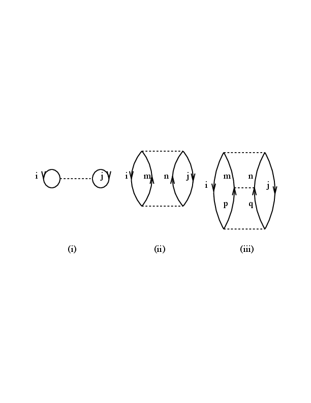
Using the standard diagram rules (see the discussion on coupled-cluster theory and many-body perturbation theory), the various
diagrams contained in the above figure can be readily calculated (in an uncoupled scheme)
$$
\begin{equation}
(i)=\frac{(-)^{n_h+n_l}}{2^{n_{ep}}}\sum_{ij\leq k_F}
\langle ij\vert\hat{v}\vert ij\rangle_{AS},
\end{equation}
$$
with \( n_h=n_l=2 \) and \( n_{ep}=1 \). As discussed in connection with the diagram rules in the many-body perturbation theory chapter, \( n_h \)
denotes the number of hole lines, \( n_l \) the number of closed
fermion loops and \( n_{ep} \) is the number of so-called
equivalent pairs.
The factor \( 1/2^{n_{ep}} \) is needed since we want to count a pair
of particles only once. We will carry this factor \( 1/2 \) with us
in the equations below.
The subscript \( AS \) denotes the antisymmetrized and normalized matrix element
$$
\begin{equation}
\langle ij\vert\hat{v}\vert ij\rangle_{AS}=\langle ij \vert\hat{v}\vert ij\rangle-
\langle ji \vert\hat{v}\vert ij\rangle.
\end{equation}
$$
Similarly, diagrams (ii) and (iii) read
$$
\begin{equation}
(ii)=\frac{(-)^{2+2}}{2^2}\sum_{ij\leq k_F}\sum_{ab>k_F}
\frac{\langle ij\vert\hat{v}\vert ab\rangle_{AS}
\langle ab\vert\hat{v}\vert ij\rangle_{AS}}
{\varepsilon_i+\varepsilon_j-\varepsilon_a-\varepsilon_b},
\end{equation}
$$
and
$$
\begin{equation}
(iii)=\frac{(-)^{2+2}}{2^3}\sum_{k_i,k_j\leq k_F}\sum_{abcdk_F}
\frac{\langle ij\vert\hat{v}\vert ab\rangle_{AS}
\langle ab\vert\hat{v}\vert cd\rangle_{AS}
\langle cd\vert\hat{v}\vert ij\rangle_{AS}}
{(\varepsilon_i+\varepsilon_j-\varepsilon_a-\varepsilon_b)
(\varepsilon_i+\varepsilon_j-\varepsilon_c-\varepsilon_d)}.
\end{equation}
$$
In the above, \( \varepsilon \) denotes the sp energies defined by
\( H_0 \).
The steps leading to the above expressions for the various
diagrams are rather straightforward. Though, if we wish to compute the
matrix elements for the interaction \( v \), a serious problem
arises. Typically, the matrix elements will contain a term
(see the next section for the formal details) \( V(|{\mathbf r}|) \), which
represents the interaction potential \( V \) between two nucleons, where
\( {\mathbf r} \) is the internucleon distance.
All modern models
for \( V \) have a strong short-range repulsive core. Hence,
matrix elements involving \( V(|{\mathbf r}|) \), will result in large
(or infinitely large for a potential with a hard core)
and repulsive contributions to the ground-state energy. Thus, the
diagrammatic expansion for the ground-state energy in terms of the
potential \( V(|{\mathbf r}|) \) becomes meaningless.
One possible solution to this problem is provided by the well-known
Brueckner theory or the Brueckner \( G \)-matrix, or just the
\( G \)-matrix. In fact, the \( G \)-matrix is an almost indispensable
tool in almost every microscopic nuclear structure
calculation. Its main idea may be paraphrased as follows.
Suppose we want to calculate the function \( f(x)=x/(1+x) \). If
\( x \) is small, we may expand the function \( f(x) \) as a power series
\( x+x^2+x^3+\dots \) and it may be adequate to just calculate the first
few terms. In other words, \( f(x) \) may be calculated using a low-order
perturbation method. But if \( x \) is large
(or infinitely large), the above
power series is obviously meaningless.
However, the exact function
\( x/(1+x) \) is still well defined in the limit
of \( x \) becoming very large.
These arguments suggest that one should sum up the diagrams
(i), (ii), (iii) in fig. 1 and the similar ones
to all orders, instead of computing them one by one. Denoting this
all-order sum as \( 1/2\tilde{G}_{ijij} \), where we have
introduced the shorthand notation
\( \tilde{G}_{ijij}=\langle k_ik_j\vert \tilde{G}\vert k_ik_j\rangle_{AS} \)
(and similarly for \( \tilde{v} \)),
we have that
$$
\begin{align}
\frac{1}{2}\tilde{G}_{ijij}=&\frac{1}{2}\hat{v}_{ijij}
+\sum_{ab>k_F}\frac{1}{2}\hat{v}_{ijab}\frac{1}{\varepsilon_i+\varepsilon_j-\varepsilon_a-\varepsilon_b}
\nonumber \\
& \times\left[\frac{1}{2}\hat{v}_{abij}+\sum_{cd>k_F}
\frac{1}{2}\hat{v}_{abcd}\frac{1}
{\varepsilon_i+\varepsilon_j-\varepsilon_c-\varepsilon_d}
\frac{1}{2}V_{cdij}+\dots \right].
\end{align}
$$
The factor \( 1/2 \) is the same as that discussed above, namely we want
to count a pair of particles only once.
The quantity inside the brackets is just
\( 1/2\tilde{G}_{mnij} \) and the above equation can be
rewritten as an integral equation
$$
\begin{equation}
\tilde{G}_{ijij}=\tilde{V}_{ijij}
+\sum_{ab>F}\frac{1}{2}\hat{v}_{ijab}\frac{1}{\varepsilon_i+\varepsilon_j-\varepsilon_a-\varepsilon_b}
\tilde{G}_{abij}.
\end{equation}
$$
Note that \( \tilde{G} \) is the antisymmetrized \( G \)-matrix since
the potential \( \tilde{v} \) is also antisymmetrized. This means that
\( \tilde{G} \) obeys
$$
\begin{equation}
\tilde{G}_{ijij}=-\tilde{G}_{jiij}=-\tilde{G}_{ijji}.
\end{equation}
$$
The \( \tilde{G} \)-matrix is defined as
$$
\begin{equation}
\tilde{G}_{ijij}=G_{ijij}-G_{jiij},
\end{equation}
$$
and the equation for \( G \) is
$$
\begin{equation}
G_{ijij}=V_{ijij}
+\sum_{ab>k_F}V_{ijab}\frac{1}
{\varepsilon_i+\varepsilon_j-\varepsilon_a-\varepsilon_b}
G_{abij},
\tag{25}
\end{equation}
$$
which is the familiar \( G \)-matrix equation. The above
matrix is specifically designed to treat a class of diagrams
contained in \( \Delta E_0 \), of which typical contributions
were shown in fig. 1. In fact the sum of the diagrams
in fig. 1 is equal to \( 1/2(G_{ijij}-G_{jiij}) \).
Let us now define a more general \( G \)-matrix as
$$
\begin{equation}
G_{ijij}=V_{ijij}
+\sum_{mn>0}V_{ijmn}\frac{Q(mn)}
{\omega -\varepsilon_m-\varepsilon_n}
G_{mnij},
\tag{26}
\end{equation}
$$
which is an extension of Eq. (25). Note that
Eq. (25) has
\( \varepsilon_i+\varepsilon_j \) in the energy denominator, whereas
in the latter equation we have a general energy variable \( \omega \)
in the denominator. Furthermore, in Eq. (25)
we have a restricted
sum over \( mn \), while in Eq. (26)
we sum over all \( ab \) and we have
introduced a weighting factor \( Q(ab) \). In Eq. (26) \( Q(ab) \)
corresponds to the choice
$$
\begin{equation}
Q(a , b ) =
\left\{\begin{array}{cc}1,&min(a ,b ) > k_F\\
0,&\mathrm{else}.\end{array}\right. ,
\end{equation}
$$
where \( Q(ab) \) is usually referred to as the \( G \)-matrix Pauli
exclusion operator. The role of \( Q \) is to enforce a selection
of the intermediate states allowed in the \( G \)-matrix equation. The above
\( Q \) requires that the intermediate particles \( a \) and \( b \)
must be both above the Fermi surface defined by \( F \). We may enforce
a different requirement by using a summation over intermediate states
different from that in Eq. (26).
An example is the Pauli operator
for the model-space Brueckner-Hartree-Fock method discussed below.
Before ending this section, let us rewrite the \( G \)-matrix equation
in a more compact form.
The sp energies \( \varepsilon \) and wave functions are defined
by the unperturbed hamiltonian \( H_0 \) as
$$
\begin{equation}
H_0\vert \psi_a\psi_b=(\varepsilon_a+\varepsilon_b)
\vert \psi_a\psi_b.
\end{equation}
$$
The \( G \)-matrix equation can then be rewritten in the following
compact form
$$
\begin{equation}
G(\omega )=V+V\frac{\hat{Q}}{\omega -H_0}G(\omega ),
\end{equation}
$$
with
\( \hat{Q}=\sum_{ab}\vert \psi_a\psi_b\langle\langle \psi_a\psi_b\vert \).
In terms of diagrams, \( G \) corresponds to an all-order sum of the
"ladder-type" interactions between two particles with the
intermediate states restricted by \( Q \).
The \( G \)-matrix equation has a very simple form. But its
calculation is rather complicated, particularly for finite
nuclear systems such as the nucleus $^{18}$O. There are a
number of complexities. To mention a few, the Pauli operator
\( Q \) may not commute with the unperturbed hamiltonian
\( H_0 \) and we have to make the replacement
$$
\frac{Q}{\omega -H_0}\rightarrow Q\frac{1}{\omega -QH_0Q}Q.
$$
The determination of the starting energy \( \omega \) is also another
problem.
In a medium such as nuclear
matter we must account
for the fact that certain states are not available as intermediate
states in the calculation of the \( G \)-matrix.
Following the discussion above
this is achieved by introducing the medium
dependent Pauli operator \( Q \). Further, the
energy \( \omega \) of the incoming particles, given by a pure kinetic
term in a scattering problem between two unbound particles (for example two colliding protons), must be modified so as to allow
for medium corrections.
How to evaluate the Pauli operator for
nuclear matter is, however, not straightforward.
Before discussing how to evaluate the Pauli operator for nuclear matter,
we note that the \( G \)-matrix
is conventionally given in terms of partial waves and
the coordinates of the relative and center-of-mass motion.
If we assume that the \( G \)-matrix is diagonal in \( \alpha \) (\( \alpha \) is a shorthand
notation for \( J \), \( S \), \( L \) and \( T \)), we write the equation for the \( G \)-matrix as a
coupled-channels equation in the relative and center-of-mass system
$$
\begin{equation}
G_{ll'}^{\alpha}(kk'K\omega )=V_{ll'}^{\alpha}(kk')
+\sum_{l''}\int \frac{d^3 q}{(2\pi )^3}V_{ll''}^{\alpha}(kq)
\frac{Q(q,K)}{\omega -H_0}
G_{l''l'}^{\alpha}(qk'K\omega).
\tag{27}
\end{equation}
$$
This equation is similar in structure to the scattering
equations discussed in connection with nuclear forces (see the chapter on models for nuclear forces), except that we now have
introduced the Pauli operator \( Q \) and a medium dependent two-particle
energy \( \omega \). The notations in this equation follow those of the chapter on nuclear forces
where we discuss the solution of the scattering
matrix \( T \).
The numerical details on how to solve the above \( G \)-matrix
equation through matrix inversion techniques are discussed below
Note however that the \( G \)-matrix may not be diagonal in \( \alpha \).
This is due to the fact that the
Pauli operator \( Q \) is not diagonal
in the above representation in the relative and center-of-mass
system. The Pauli operator depends on the
angle between the relative momentum and the center of mass momentum.
This angle dependence causes \( Q \) to couple states with different
relative angular
momentua \( {\cal J} \), rendering a partial wave decomposition of the \( G \)-matrix equation
rather difficult.
The angle dependence of the Pauli operator
can be eliminated by introducing the angle-average
Pauli operator, where one replaces the exact Pauli operator \( Q \)
by its average \( \bar{Q} \) over all angles for fixed relative and center-of-mass
momenta.
The choice of Pauli operator is decisive to the determination of the
sp
spectrum. Basically, to first order in the reaction matrix \( G \),
there are three commonly used sp spectra, all
defined by the solution of the following equations
$$
\begin{equation}
\varepsilon_{m} = \varepsilon (k_{m})= t_{m} + u_{m}=\frac{k_{m}^2}{2M_N}+u_{m},
\tag{28}
\end{equation}
$$
and
$$
\begin{align}
u_{m} =& {\displaystyle \sum_{h \leq k_F}}\left\langle m h \right| G(\omega = \varepsilon_{m} + \varepsilon_h )
\left| m h \right\rangle_{AS} \hspace{3mm}k_m \leq k_M, \\ \\
u_m=&0, k_m > k_M.
\tag{29}
\end{align}
$$
For notational economy, we set \( |{\bf k}_m|=k_m \).
Here we employ antisymmetrized matrix elements (AS), and \( k_M \) is a cutoff
on the momentum. Further, \( t_m \) is the sp kinetic
energy and similarly \( u_m \)
is the
sp potential.
The choice of cutoff \( k_M \) is actually what determines the three
commonly used sp spectra.
In the conventional BHF approach one employs \( k_M = k_F \),
which leads
to a Pauli operator \( Q_{\mathrm{BHF}} \) (in the laboratory system) given by
$$
\begin{equation}
Q_{\mathrm{BHF}}(k_m , k_n ) =
\left\{\begin{array}{cc}1,&min(k_m ,k_n ) > k_F\\
0,&\mathrm{else}.\end{array}\right.
\tag{30},
\end{equation}
$$
or, since we will define an
angle-average Pauli operator in the relative and center-of-mass
system, we have
$$
\begin{equation}
\bar{Q}_{\mathrm{BHF}}(k,K)=\left\{\begin{array}{cc}
0,&k\leq \sqrt{k_{F}^{2}-K^2/4}\\
1,&k\geq k_F + K/2\\
\frac{K^2/4+k^2 -k_{F}^2}{kK}&\mathrm{else},\end{array}\right.
\tag{31}
\end{equation}
$$
with \( k_F \) the momentum at the Fermi surface.
The BHF choice sets \( u_k = 0 \) for \( k > k_F \), which leads
to an unphysical, large gap at the Fermi surface, typically
of the order of \( 50-60 \) MeV.
To overcome the gap
problem, Mahaux and collaborators
introduced a continuous sp spectrum
for all values of \( k \). The divergencies
which then may occur in Eq. (27) are taken care of by
introducing
a principal value integration in Eq. (27),
to retain only the
real part contribution to the \( G \)-matrix.
To define the energy denominators we will also make use of the
angle-average approximation.
The angle dependence is handled by the
so-called effective mass approximation. The single-particle energies
in nuclear matter are assumed to have the simple quadratic form
$$
\begin{equation}
\begin{array}{ccc}
\varepsilon (k_m)=&
{\displaystyle\frac{\hbar^{2}k_m^2}
{2M_{N}^{*}}}+\Delta ,&\hspace{3mm}k_m\leq k_F\\
&&\\
=&{\displaystyle\frac{\hbar^{2}
k_m^2}{2M_{N}}},&\hspace{3mm}k_m> k_F ,\\
\end{array}
\tag{32}
\end{equation}
$$
where \( M_{N}^{*} \) is the effective mass of the nucleon and \( M_{N} \) is the
bare nucleon mass. For particle states above the Fermi sea we choose
a pure kinetic energy term, whereas for hole states,
the terms \( M_{N}^{*} \) and \( \Delta \), the latter being
an effective single-particle
potential related to the \( G \)-matrix, are obtained through the
self-consistent Brueckner-Hartree-Fock procedure.
The sp potential is obtained through the same angle-average approximation
$$
\begin{align}
\tag{33}
U(k_m) & =\sum_{l\alpha} (2T+1)(2J+1)
\left \{ \frac{8}{\pi}\int_{0}^{(k_F-k_m)/2}
k^2dk G_{ll}^{\alpha}(k,\bar{K}_1) \right. \\
& \left.
+ \frac{1}{\pi k_m}\int_{(k_F-k_m)/2}^{(k_F+k_m)/2}
kdk (k_F ^2-(k_m-2k)^2)
G_{ll}^{\alpha}(k,\bar{K}_2) \right \} \nonumber,
\end{align}
$$
where we have defined
$$
\begin{equation}
\bar{K}_1^2=4(k_m^2+k^2),
\end{equation}
$$
and
$$
\begin{equation}
\bar{K}_2^2=4(k_m^2+k^2)-(2k+k_m-k_F)(2k+k_1+k_F).
\end{equation}
$$
This
self-consistency scheme consists in choosing adequate initial values of the
effective mass and \( \Delta \). The obtained \( G \)-matrix is in turn used to
obtain new values for \( M_{N}^{*} \) and \( \Delta \). This procedure
continues until these parameters vary little.
Exercise 4: Magic numbers for infinite matter and the Minnesota interaction model
a)
Set up the quantum numbers for infinite nuclear matter and neutron matter using a given value
of \( n_{\mathrm{max}} \).
Solution.
The following python code sets up the quantum numbers for both infinite nuclear matter and neutron matter meploying a cutoff in the value of \( n \).
from numpy import *

nmax =2
nshell = 3*nmax*nmax
count = 1
tzmin = 1

print "Symmetric nuclear matter:"
print "a, nx,   ny,   nz,   sz,   tz,   nx^2 + ny^2 + nz^2"
for n in range(nshell):
    for nx in range(-nmax,nmax+1):
         for ny in range(-nmax,nmax+1):
            for nz in range(-nmax, nmax+1):
                for sz in range(-1,1+1):
                    tz = 1
                    for tz in range(-tzmin,tzmin+1):
                        e = nx*nx + ny*ny + nz*nz
                        if e == n:
                            if sz != 0:
                                if tz != 0:
                                    print count, "  ",nx,"  ",ny, "  ",nz,"  ",sz,"  ",tz,"         ",e
                                    count += 1


nmax =1
nshell = 3*nmax*nmax
count = 1
tzmin = 1
print "------------------------------------"
print "Neutron matter:"
print "a, nx,   ny,   nz,   sz,    nx^2 + ny^2 + nz^2"
for n in range(nshell):
    for nx in range(-nmax,nmax+1):
         for ny in range(-nmax,nmax+1):
            for nz in range(-nmax, nmax+1):
                for sz in range(-1,1+1):
                    e = nx*nx + ny*ny + nz*nz
                    if e == n:
                        if sz != 0:
                            print count, "  ",nx,"  ",ny, "  ",sz,"  ",tz,"         ",e
                            count += 1