The Coupled Cluster Method
Thomas Papenbrock
The University of Tennessee, Knoxville, tpapenbr@utk.edu
Aug 4, 2018
Table of contents
The Coupled-Cluster Method
Introduction
The normal-ordered Hamiltonian
Exercise 1: Practice in normal ordering
Exercise 2: What does "good" mean?
Exercise 3: How many nuclei are accessible with the coupled cluster method based on spherical mean fields?
The similarity transformed Hamiltonian
Exercise 4: What \( T \) leads to Hermitian \( \overline{H_N} \) ?
Exercise 5: Understanding (non-unitary) similarity transformations
Exercise 6: How many unknowns?
Exercise 7: Why is CCD not exact?
Computing the similarity-transformed Hamiltonian
Exercise 8: When does CCSD truncate?
Exercise 9: Compute the matrix element \( \overline{H}_{ab}^{ij}\equiv \langle ij\vert \overline{H_N}\vert ab\rangle \)
Example: The contribution of \( [F, T_2] \) to \( \overline{H_N} \)
Exercise 10: Assign the correct matrix element \( \langle pq\vert V\vert rs\rangle \) to each of the following diagrams of the interaction
Example: CCSD correlation energy
CCD Approximation
Exercise 11: Derive the CCD equations!
Exercise 12: Computational scaling of CCD
Exercise 13: Factorize the remaining diagrams of the CCD equation
Project 14: (Optional) Derive the CCSD equations!
Solving the CCD equations
CCD for the pairing Hamiltonian
Project 15: Solve the CCD equations for the pairing problem
Nucleonic Matter
Exercise 16: Which symmetries are relevant for nuclear matter?
Basis states
Exercise 17: Determine the basis states
Exercise 18: How large should the basis be?
Exercise 19: Determine the lowest few magic numbers for a cubic lattice.
Finite size effects
Channel structure of Hamiltonian and cluster amplitudes
Example: Channel structure and its usage
Exercise 20: Write a CCD code for neutron matter, focusing first on ladder approximation, i.e. including the first five diagrams in Figure 11.
Benchmarks with the Minnesota potential
From Structure to Reactions
Electroweak reactions
Computing optical potentials from microscopic input
The Coupled-Cluster Method
Introduction
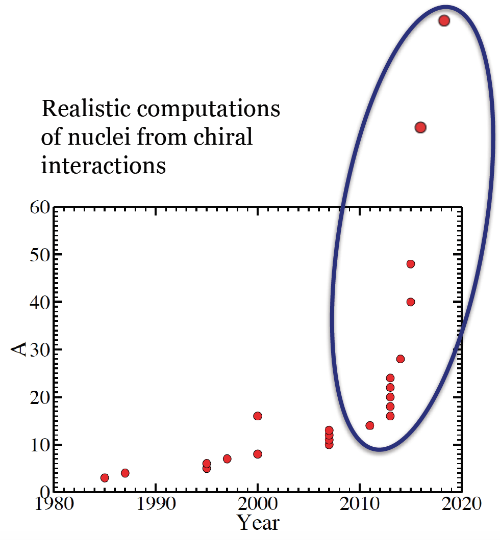
The coupled-cluster method is an efficient tool to compute atomic
nuclei with an effort that grows polynomial with system size. While
this might still be expensive, it is now possible to compute nuclei
with mass numbers about \( A\approx 100 \) with this method. Recall that
full configuration interaction (FCI) such as the no-core shell model
exhibits an exponential cost and is therefore limited to light nuclei.
Figure 1: Realistic computations of atomic nuclei with interactions from chiral EFT. The slow increase prior to 2015 is based on quantum Monte Carlo and the no-core shell model. These methods are exponentially expensive (in mass number \( A \)) and meet with exponentially increasing computer power (Moore's law), thus leading to a progress that is linear in time. Methods such as coupled clusters and in-medium SRG carry a polynomial cost in mass number are transforming the field.
The normal-ordered Hamiltonian
We start from the reference state
$$
\begin{equation}
\label{HFref}
\vert\Phi_0\rangle = \prod_{i=1}^A a^\dagger_i \vert 0\rangle
\end{equation}
$$
for the description of a nucleus with mass number \( A \). Usually, this
reference is the Hartree-Fock state, but that is not necessary. In the
shell-model picture, it could also be a product state where the lowest
\( A \) harmonic oscillator states are occupied. Here and in what
follows, the indices \( i,j,k,\ldots \) run over hole states,
i.e. orbitals occupied in the reference state \eqref{HFref}, while
\( a,b,c,\ldots \) run over particle states, i.e. unoccupied
orbitals. Indices \( p,q,r,s \) can identify any orbital. Let \( n_u \) be
the number of unoccupied states, and \( A \) is of course the number of
occupied states. We consider the Hamiltonian
$$
\begin{equation}
\label{Ham} H =
\sum_{pq} \varepsilon^p_q a^\dagger_p a_q +
\frac{1}{4}\sum_{pqrs}\langle pq\vert V\vert rs\rangle
a^\dagger_pa^\dagger_q a_sa_r
\end{equation}
$$
The reference state \eqref{HFref} is a non-trivial vacuum of our theory.
We normal order this Hamiltonian with respect to the nontrivial vacuum
state given by the Hartree-Fock reference and obtain the
normal-ordered Hamiltonian
$$
\begin{equation}
\label{HN}
H_N = \sum_{pq} f_{pq} \left\{a^\dagger_p a_q\right\} + \frac{1}{4}\sum_{pqrs}\langle pq\vert V\vert rs\rangle \left\{a^\dagger_pa^\dagger_q a_sa_r\right\}.
\end{equation}
$$
Here,
$$
\begin{equation}
\label{Fock}
f^p_q = \varepsilon^p_q + \sum_i \langle pi\vert V\vert qi\rangle
\end{equation}
$$
is the Fock matrix. We note that the Fock matrix is diagonal in the
Hartree-Fock basis. The brackets \( \{\cdots\} \) in Eq. \eqref{HN} denote
normal ordering, i.e. all operators that annihilate the nontrivial
vaccum \eqref{HFref} are to the right of those operators that create
with respect to that vaccum. Normal ordering implies that \( \langle
\Phi_0\vert H_N\vert \Phi_0\rangle = 0 \).
Exercise 1: Practice in normal ordering
Normal order the expression \( \sum\limits_{pq}\varepsilon_q^p a^\dagger_p a_q \).
Hint.
$$
\begin{align}
\sum_{pq}\varepsilon_q^p a^\dagger_p a_q
=\sum_{ab}\varepsilon_b^a a^\dagger_a a_b
+\sum_{ai}\varepsilon_i^a a^\dagger_a a_i
+\sum_{ai}\varepsilon_a^i a^\dagger_i a_a
+\sum_{ij}\varepsilon_j^i a^\dagger_i a_j
\label{_auto1}
\end{align}
$$
Answer.
We have to move all operators that annihilate the reference state to the right of those that create on the reference state. Thus,
$$
\begin{align}
\sum_{pq}\varepsilon_q^p a^\dagger_p a_q
&=\sum_{ab}\varepsilon_b^a a^\dagger_a a_b
+\sum_{ai}\varepsilon_i^a a^\dagger_a a_i
+\sum_{ai}\varepsilon_a^i a^\dagger_i a_a
+\sum_{ij}\varepsilon_j^i a^\dagger_i a_j
\label{_auto2}\\
&=\sum_{ab}\varepsilon_b^a a^\dagger_a a_b
+\sum_{ai}\varepsilon_i^a a^\dagger_a a_i
+\sum_{ai}\varepsilon_a^i a^\dagger_i a_a
+\sum_{ij}\varepsilon_j^i \left(-a_ja^\dagger_i +\delta_i^j\right)
\label{_auto3}\\
&=\sum_{ab}\varepsilon_b^a a^\dagger_a a_b
+\sum_{ai}\varepsilon_i^a a^\dagger_a a_i
+\sum_{ai}\varepsilon_a^i a^\dagger_i a_a
-\sum_{ij}\varepsilon_j^i a_ja^\dagger_i +\sum_i \varepsilon_i^i
\label{_auto4}\\
&=\sum_{pq}\varepsilon_q^p \left\{a^\dagger_p a_q\right\} +\sum_i \varepsilon_i^i
\label{_auto5}
\end{align}
$$
We note that \( H = E_{HF} + H_N \), where
$$
\begin{align}
E_{HF} &\equiv \langle\Phi_0\vert H\vert \Phi_0\rangle = \sum_{i} \varepsilon^i_i +\frac{1}{2}\sum_{ij}\langle ij\vert V\vert ij\rangle
\label{_auto6}
\end{align}
$$
is the Hartree-Fock energy.
The coupled-cluster method is a very efficient tool to compute nuclei
when a "good" reference state is available. Let us assume that the
reference state results from a Hartree-Fock calculation.
Exercise 2: What does "good" mean?
How do you know whether a Hartree-Fock state is a "good" reference?
Which results of the Hartree-Fock computation will inform you?
Answer.
Once the Hartree-Fock equations are solved, the Fock matrix
\eqref{Fock} becomes diagonal, and its diagonal elements can be viewed
as single-particle energies. Hopefully, there is a clear gap in the
single-particle spectrum at the Fermi surface, i.e. after \( A \) orbitals
are filled.
If symmetry-restricted Hartree-Fock is used, one is limited to compute
nuclei with closed subshells for neutrons and for protons. On a first
view, this might seem as a severe limitation. But is it?
Exercise 3: How many nuclei are accessible with the coupled cluster method based on spherical mean fields?
If one limits oneself to nuclei with mass number up to
mass number \( A=60 \), how many nuclei can potentially be described with
the coupled-cluster method? Which of these nuclei are potentially
interesting? Why?
Answer.
Nuclear shell closures are at \( N,Z=2,8,20,28,50,82,126 \), and subshell
closures at \( N,Z=2,6,8,14,16,20,28,32,34,40,50,\ldots \).
In the physics of nuclei, the evolution of nuclear structure as
neutrons are added (or removed) from an isotope is a key
interest. Examples are the rare isotopes of helium (He-8,10)
oxygen (O-22,24,28), calcium (Ca-52,54,60), nickel (Ni-78) and tin
(Sn-100,132). The coupled-cluster method has the
potential to address questions regarding these nuclei, and in a
several cases was used to make predictions before experimental data
was available. In addition, the method can be used to compute
neighbors of nuclei with closed subshells.
The similarity transformed Hamiltonian
There are several ways to view and understand the coupled-cluster
method. A first simple view of coupled-cluster theory is that the
method induces correlations into the reference state by expressing a
correlated state as
$$
\begin{equation}
\label{psi}
\vert\Psi\rangle = e^T \vert\Phi_0\rangle ,
\end{equation}
$$
Here, \( T \) is an operator that induces correlations. We can now demand
that the correlate state \eqref{psi} becomes and eigenstate of the
Hamiltonian \( H_N \), i.e. \( H_N\vert \Psi\rangle = E\vert \Psi\rangle \). This view,
while correct, is not the most productive one. Instead, we
left-multiply the Schroedinger equation with \( e^{-T} \) and find
$$
\begin{equation}
\label{Schroedinger}
\overline{H_N}\vert \Phi_0\rangle = E_c \vert \Phi_0\rangle .
\end{equation}
$$
Here, \( E_c \) is the correlation energy, and the total energy is
\( E=E_c+E_{HF} \). The similarity-transformed Hamiltonian is defined as
$$
\begin{equation}
\label{Hsim}
\overline{H_N} \equiv e^{-T} H_N e^T .
\end{equation}
$$
A more productive view on coupled-cluster theory thus emerges: This
method seeks a similarity transformation such that the uncorrelated
reference state \eqref{HFref} becomes an exact eigenstate of the
similarity-transformed Hamiltonian \eqref{Hsim}.
Exercise 4: What \( T \) leads to Hermitian \( \overline{H_N} \) ?
What are the conditions on \( T \) such that \( \overline{H_N} \) is Hermitian?
Answer.
For a Hermitian \( \overline{H_N} \), we need a unitary \( e^T \), i.e. an
anti-Hermitian \( T \) with \( T = -T^\dagger \)
As we will see below, coupld-cluster theory employs a non-Hermitian Hamiltonian.
Exercise 5: Understanding (non-unitary) similarity transformations
Show that \( \overline{H_N} \) has the same eigenvalues as \( H_N \) for
arbitrary \( T \). What is the spectral decomposition of a non-Hermitian
\( \overline{H_N} \) ?
Answer.
Let \( H_N\vert E\rangle = E\vert E\rangle \). Thus
$$
\begin{align*}
H_N e^{T} e^{-T} \vert E\rangle &= E\vert E\rangle , \\
\left(e^{-T} H_N e^T\right) e^{-T} \vert E\rangle &= Ee^{-T} \vert E\rangle , \\
\overline{H_N} e^{-T} \vert E\rangle &= E e^{-T}\vert E\rangle .
\end{align*}
$$
Thus, if \( \vert E\rangle \) is an eigenstate of \( H_N \) with eigenvalue \( E \),
then \( e^{-T}\vert E\rangle \) is eigenstate of \( \overline{H_N} \) with the same
eigenvalue.
A non-Hermitian \( \overline{H_N} \) has eigenvalues \( E_\alpha \)
corresponding to left \( \langle L_\alpha\vert \) and right \( \vert R_\alpha
\rangle \) eigenstates. Thus
$$
\begin{align}
\overline{H_N} = \sum_\alpha \vert R_\alpha\rangle E_\alpha \langle L_\alpha \vert
\label{_auto7}
\end{align}
$$
with bi-orthonormal \( \langle L_\alpha\vert R_\beta\rangle = \delta_\alpha^\beta \).
To make progress, we have to specify the cluster operator \( T \). In
coupled cluster theory, this operator is
$$
\begin{equation}
\label{Top}
T \equiv \sum_{ia} t_i^a a^\dagger_a a_i + \frac{1}{4}\sum_{ijab}t_{ij}^{ab}
a^\dagger_aa^\dagger_ba_ja_i + \cdots
+ \frac{1}{(A!)^2}\sum_{i_1\ldots i_A a_1 \ldots a_A}
t_{i_1\ldots i_A}^{a_1\ldots a_A} a^\dagger_{a_1}\cdots a^\dagger_{a_A} a_{i_A}\cdots a_{i_1} .
\end{equation}
$$
Thus, the operator \eqref{Top} induces particle-hole (p-h)
excitations with respect to the reference. In general, \( T \) generates
up to \( Ap-Ah \) excitations, and the unknown parameters are the cluster amplitides
\( t_i^a \), \( t_{ij}^{ab} \), ..., \( t_{i_1,\ldots,i_A}^{a_1,\ldots,a_A} \).
Exercise 6: How many unknowns?
Show that the number of unknowns is as large as the FCI dimension of
the problem, using the numbers \( A \) and \( n_u \).
Answer.
We have to sum up all \( np-nh \) excitations, and there are
\( \binom{n_u}{n} \) particle states and \( \binom{A}{A-n} \) hole states for
each \( n \). Thus, we have for the total number
$$
\begin{align}
\sum_{n=0}^A \binom{n_u}{n} \binom{A}{A-n}= \binom{A+n_u}{A} .
\label{_auto8}
\end{align}
$$
The right hand side are obviously all ways to distribute \( A \) fermions over \( n_0+A \) orbitals.
Thus, the coupled-cluster method with the full cluster operator
\eqref{Top} is exponentially expensive, just as FCI. To make progress,
we need to make an approximation by truncating the operator. Here, we
will use the CCSD (coupled clusters singles doubles) approximation,
where
$$
\begin{equation}
\label{Tccsd}
T \equiv \sum_{ia} t_i^a a^\dagger_a a_i + \frac{1}{4}\sum_{ijab}t_{ij}^{ab}
a^\dagger_aa^\dagger_ba_ja_i .
\end{equation}
$$
We need to determine the unknown cluster amplitudes that enter in CCSD. Let
$$
\begin{align}
\vert\Phi_i^a\rangle &= a^\dagger_a a_i \vert \Phi_0\rangle ,
\label{_auto9}\\
\vert\Phi_{ij}^{ab}\rangle &= a^\dagger_a a^\dagger_b a_j a_i \vert \Phi_0\rangle
\label{_auto10}
\end{align}
$$
be 1p-1h and 2p-2h excitations of the reference. Computing matrix
elements of the Schroedinger Equation \eqref{Schroedinger} yields
$$
\begin{align}
\label{ccsd}
\langle \Phi_0\vert \overline{H_N}\vert \Phi_0\rangle &= E_c , \\
\langle \Phi_i^a\vert \overline{H_N}\vert \Phi_0\rangle &= 0 ,
\label{_auto11}\\
\langle \Phi_{ij}^{ab}\vert \overline{H_N}\vert \Phi_0\rangle &= 0 .
\label{_auto12}
\end{align}
$$
The first equation states that the coupled-cluster correlation energy
is an expectation value of the similarity-transformed Hamiltonian. The
second and third equations state that the similarity-transformed
Hamiltonian exhibits no 1p-1h and no 2p-2h excitations. These
equations have to be solved to find the unknown amplitudes \( t_i^a \) and
\( t_{ij}^{ab} \). Then one can use these amplitudes and compute the
correlation energy from the first line of Eq. \eqref{ccsd}.
We note that in the CCSD approximation the reference state is not an
exact eigenstates. Rather, it is decoupled from simple states but
\( \overline{H} \) still connects this state to 3p-3h, and 4p-4h states
etc.
At this point, it is important to recall that we assumed starting from
a "good" reference state. In such a case, we might reasonably expect
that the inclusion of 1p-1h and 2p-2h excitations could result in an
accurate approximation. Indeed, empirically one finds that CCSD
accounts for about 90% of the corelation energy, i.e. of the
difference between the exact energy and the Hartree-Fock energy. The
inclusion of triples (3p-3h excitations) typically yields 99% of the
correlation energy.
We see that the coupled-cluster method in its CCSD approximation
yields a similarity-transformed Hamiltonian that is of a two-body
structure with respect to a non-trivial vacuum. When viewed in this
light, the coupled-cluster method "transforms" an \( A \)-body problem
(in CCSD) into a two-body problem, albeit with respect to a nontrivial
vacuum.
Exercise 7: Why is CCD not exact?
Above we argued that a similarity transformation preserves all eigenvalues. Nevertheless, the CCD correlation energy is not the exact correlation energy. Explain!
Answer.
The CCD approximation does not make \( \vert\Phi_0\rangle \) an exact
eigenstate of \( \overline{H_N} \); it is only an eigenstate when the
similarity-transformed Hamiltonian is truncated to at most 2p-2h
states. The full \( \overline{H_N} \), with \( T=T_2 \), would involve
six-body terms (do you understand this?), and this full Hamiltonian
would reproduce the exact correlation energy. Thus CCD is a similarity
transformation plus a truncation, which decouples the ground state only
from 2p-2h states.
Computing the similarity-transformed Hamiltonian
The solution of the CCSD equations, i.e. the second and third line of
Eq. \eqref{ccsd}, and the computation of the correlation energy
requires us to compute matrix elements of the similarity-transformed
Hamiltonian \eqref{Hsim}. This can be done with the
Baker-Campbell-Hausdorff expansion
$$
\begin{align}
\label{BCH}
\overline{H_N} &= e^{-T} H_N e^T \\
&=H_N + \left[ H_N, T\right]+ \frac{1}{2!}\left[ \left[ H_N, T\right], T\right]
+ \frac{1}{3!}\left[\left[ \left[ H_N, T\right], T\right], T\right] +\ldots .
\label{_auto13}
\end{align}
$$
We now come to a key element of coupled-cluster theory: the cluster
operator \eqref{Top} consists of sums of terms that consist of particle
creation and hole annihilation operators (but no particle annihilation
or hole creation operators). Thus, all terms that enter \( T \) commute
with each other. This means that the commutators in the
Baker-Campbell-Hausdorff expansion \eqref{BCH} can only be non-zero
because each \( T \) must connect to \( H_N \) (but no \( T \) with another
\( T \)). Thus, the expansion is finite.
Exercise 8: When does CCSD truncate?
In CCSD and for two-body Hamiltonians, how many nested
commutators yield nonzero results? Where does the
Baker-Campbell-Hausdorff expansion terminate? What is the (many-body) rank of the resulting \( \overline{H_N} \)?
Answer.
CCSD truncates for two-body operators at four-fold nested commutators,
because each of the four annihilation and creation operators in
\( \overline{H_N} \) can be knocked out with one term of \( T \).
We see that the (disadvantage of having a) non-Hermitian Hamiltonian
\( \overline{H_N} \) leads to the advantage that the
Baker-Campbell-Hausdorff expansion is finite, thus leading to the
possibility to compute \( \overline{H_N} \) exactly. In contrast, the
IMSRG deals with a Hermitian Hamiltonian throughout, and the infinite
Baker-Campbell-Hausdorff expansion is truncated at a high order when
terms become very small.
We write the similarity-transformed Hamiltonian as
$$
\begin{align}
\overline{H_N}=\sum_{pq} \overline{H}^p_q a^\dagger_q a_p + {1\over 4} \sum_{pqrs} \overline{H}^{pq}_{rs} a^\dagger_p a^\dagger_q a_s a_r + \ldots
\label{_auto14}
\end{align}
$$
with
$$
\begin{align}
\overline{H}^p_q &\equiv \langle p\vert \overline{H_N}\vert q\rangle ,
\label{_auto15}\\
\overline{H}^{pq}_{rs} &\equiv \langle pq\vert \overline{H_N}\vert rs\rangle .
\label{_auto16}
\end{align}
$$
Thus, the CCSD Eqs. \eqref{ccsd} for the amplitudes can be written as
\( \overline{H}_i^a = 0 \) and \( \overline{H}_{ij}^{ab}=0 \).
Exercise 9: Compute the matrix element \( \overline{H}_{ab}^{ij}\equiv \langle ij\vert \overline{H_N}\vert ab\rangle \)
Answer.
This is a simple task. This matrix element is part of the operator
\( \overline{H}_{ab}^{ij}a^\dagger_ia^\dagger_ja_ba_a \), i.e. particles
are annihilated and holes are created. Thus, no contraction of the
Hamiltonian \( H \) with any cluster operator \( T \) (remember that \( T \)
annihilates holes and creates particles) can happen, and we simply
have \( \overline{H}_{ab}^{ij} = \langle ij\vert V\vert ab\rangle \).
We need to work out the similarity-transformed Hamiltonian of
Eq. \eqref{BCH}. To do this, we write \( T=T_1 +T_2 \) and \( H_N= F +V \),
where \( T_1 \) and \( F \) are one-body operators, and \( T_2 \) and \( V \) are
two-body operators.
Example: The contribution of \( [F, T_2] \) to \( \overline{H_N} \)
The commutator \( [F, T_2] \) consists of two-body and one-body terms. Let
us compute first the two-body term, as it results from a single
contraction (i.e. a single application of \( [a_p, a^\dagger_q] =
\delta_p^q \)). We denote this as \( [F, T_2]_{2b} \) and find
$$
\begin{align*}
[F, T_2]_{2b} &= \frac{1}{4}\sum_{pq}\sum_{rsuv} f_p^q t_{ij}^{ab}\left[a^\dagger_q a_p, a^\dagger_a a^\dagger_b a_j a_i \right]_{2b} \\
&= \frac{1}{4}\sum_{pq}\sum_{abij} f_p^q t_{ij}^{ab}\delta_p^a a^\dagger_q a^\dagger_b a_j a_i \\
&- \frac{1}{4}\sum_{pq}\sum_{abij} f_p^q t_{ij}^{ab}\delta_p^b a^\dagger_q a^\dagger_a a_j a_i \\
&- \frac{1}{4}\sum_{pq}\sum_{abij} f_p^q t_{ij}^{ab}\delta_q^j a^\dagger_a a^\dagger_b a_p a_i \\
&+ \frac{1}{4}\sum_{pq}\sum_{abij} f_p^q t_{ij}^{ab}\delta_q^i a^\dagger_a a^\dagger_b a_p a_j \\
&= \frac{1}{4}\sum_{qbij}\left(\sum_{a} f_a^q t_{ij}^{ab}\right)a^\dagger_q a^\dagger_b a_j a_i \\
&- \frac{1}{4}\sum_{qaij}\left(\sum_{b} f_b^q t_{ij}^{ab}\right)a^\dagger_q a^\dagger_a a_j a_i \\
&- \frac{1}{4}\sum_{pabi}\left(\sum_{j} f_p^j t_{ij}^{ab}\right)a^\dagger_a a^\dagger_b a_p a_i \\
&+ \frac{1}{4}\sum_{pabj}\left(\sum_{i} f_p^i t_{ij}^{ab}\right)a^\dagger_a a^\dagger_b a_p a_j \\
&= \frac{1}{2}\sum_{qbij}\left(\sum_{a} f_a^q t_{ij}^{ab}\right)a^\dagger_q a^\dagger_b a_j a_i \\
&- \frac{1}{2}\sum_{pabi}\left(\sum_{j} f_p^j t_{ij}^{ab}\right)a^\dagger_a a^\dagger_b a_p a_i .
\end{align*}
$$
Here we exploited the antisymmetry \( t_{ij}^{ab} = -t_{ji}^{ab} =
-t_{ij}^{ba} = t_{ji}^{ba} \) in the last step. Using \( a^\dagger_q a^\dagger_b a_j a_i = -a^\dagger_b a^\dagger_q a_j a_i \) and \( a^\dagger_a a^\dagger_b a_p a_i = a^\dagger_a a^\dagger_b a_i a_p \), we can make the expression
manifest antisymmetric, i.e.
$$
\begin{align*}
[F, T_2]_{2b}
&= \frac{1}{4}\sum_{qbij}\left[\sum_{a} \left(f_a^q t_{ij}^{ab}-f_a^b t_{ij}^{qa}\right)\right]a^\dagger_q a^\dagger_b a_j a_i \\
&- \frac{1}{4}\sum_{pabi}\left[\sum_{j} \left(f_p^j t_{ij}^{ab}-f_i^j t_{pj}^{ab}\right)\right]a^\dagger_a a^\dagger_b a_p a_i .
\end{align*}
$$
Thus, the contribution of \( [F, T_2]_{2b} \) to the matrix element \( \overline{H}_{ij}^{ab} \) is
$$
\begin{align*}
\overline{H}_{ij}^{ab} \leftarrow \sum_{c} \left(f_c^a t_{ij}^{cb}-f_c^b t_{ij}^{ac}\right) - \sum_{k} \left(f_j^k t_{ik}^{ab}-f_i^k t_{jk}^{ab}\right)
\end{align*}
$$
Here we used an arrow to indicate that this is just one contribution
to this matrix element. We see that the derivation straight forward,
but somewhat tedious. As no one likes to commute too much (neither in
this example nor when going to and from work), and so we need a better
approach. This is where diagramms come in handy.
Diagrams
The pictures in this Subsection are taken from Crawford and Schaefer.
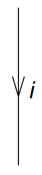
By convention, hole lines (labels \( i, j, k,\ldots \)) are pointing down.
Figure 2: This is a hole line.
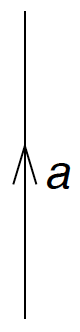
By convention, particle lines (labels \( a, b, c,\ldots \)) are pointing up.
Figure 3: This is a particle line.
Let us look at the one-body operator of the normal-ordered Hamiltonian, i.e. Fock matrix. Its diagrams are as follows.
Figure 4: The diagrams corresponding to \( f_a^b \). The dashed line with the 'X' denotes the interaction \( F \) between the incoming and outgoing lines. The labels \( a \) and \( b \) are not denoted, but you should label the outgoing and incoming lines accordingly.
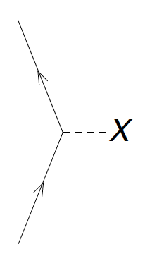
Figure 5: The diagrams corresponding to \( f_i^j \). The dashed line with the 'X' denotes the interaction \( F \) between the incoming and outgoing lines.
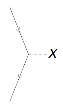
Figure 6: The diagrams corresponding to \( f_a^i \). The dashed line with the 'X' denotes the interaction \( F \) between the incoming and outgoing lines.
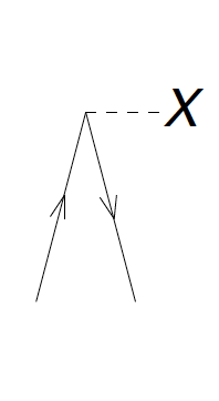
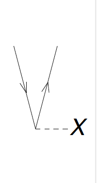
Figure 7: The diagrams corresponding to \( f_i^a \). The dashed line with the 'X' denotes the interaction \( F \) between the incoming and outgoing lines.
We now turn to the two-body interaction. It is denoted as a horizontal
dashed line with incoming and outgoing lines attached to it. We start
by noting that the following diagrams of the interaction are all
related by permutation symmetry.
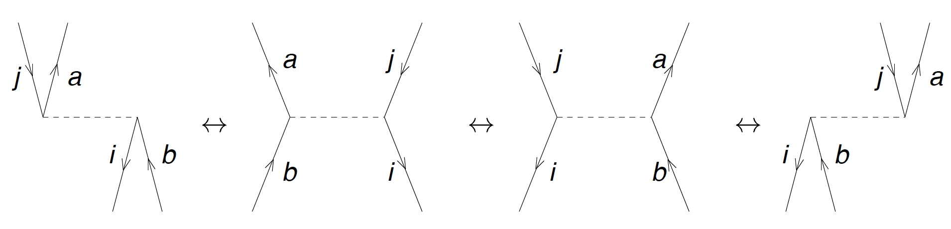
Figure 8: The diagrams corresponding to \( \langle ai\vert V\vert jb \rangle = - \langle ai\vert V\vert bj \rangle = -\langle ia\vert V\vert jb \rangle = \langle ia\vert V\vert bj\rangle \).
Exercise 10: Assign the correct matrix element \( \langle pq\vert V\vert rs\rangle \) to each of the following diagrams of the interaction
Remember: \( \langle\rm{left-out, right-out}\vert V\vert \rm{left-in, right-in}\rangle \).
a)
Answer.
\( \langle ab\vert V\vert cd\rangle + \langle ij\vert V\vert kl\rangle + \langle ia\vert V\vert bj\rangle \)
b)
Answer.
\( \langle ai\vert V\vert bc\rangle + \langle ij\vert V\vert ka\rangle + \langle ab\vert V\vert ci\rangle \)
c)
Answer.
\( \langle ia\vert V\vert jk\rangle + \langle ab\vert V\vert ij\rangle + \langle ij\vert V\vert ab\rangle \)
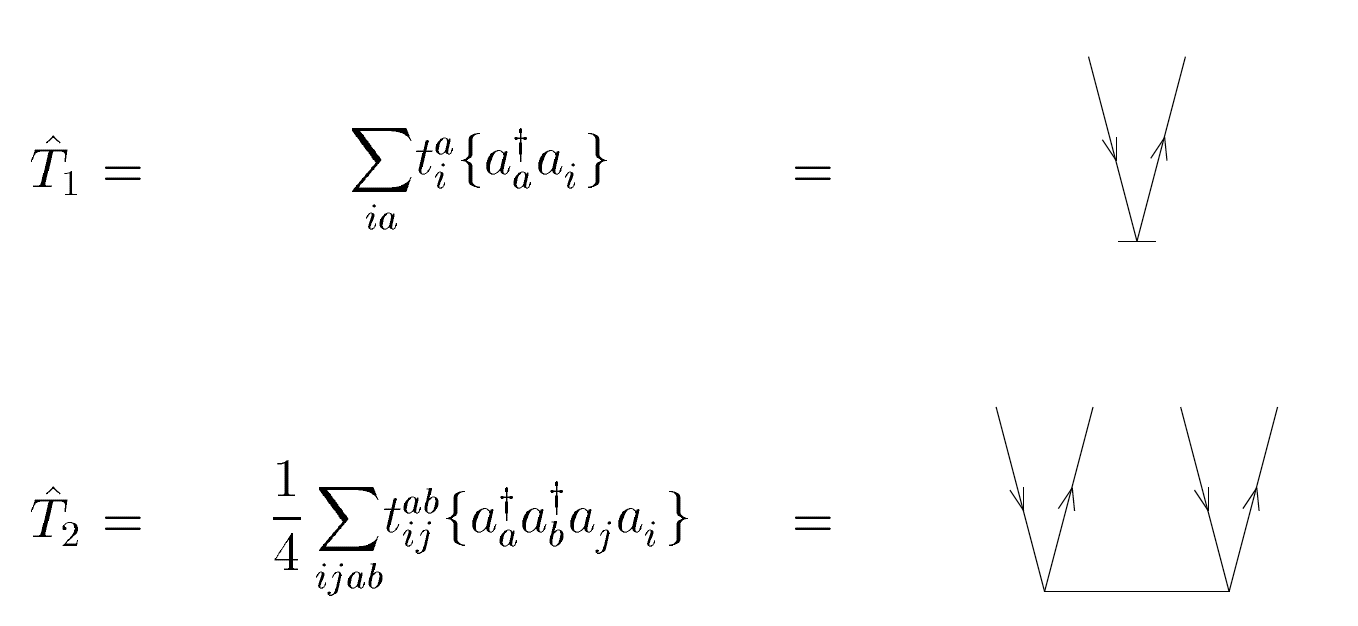
Finally, we have the following diagrams for the \( T_1 \) and \( T_2 \) amplitudes.
Figure 9: The horizontal full line is the cluster amplitude with incoming hole lines and outgoing particle lines as indicated.
We are now in the position to construct the diagrams of the
similarity-transformed Hamiltonian, keeping in mind that these
diagrams correspond to matrix elements of \( \overline{H_N} \). The rules
are as follows.
- Write down all topologically different diagrams corresponding to the desired matrix element. Topologically different diagrams differ in the number and type of lines (particle or hole) that connect the Fock matrix \( F \) or the interaction \( V \) to the cluster amplitudes \( T \), but not whether these connections are left or right (as those are related by antisymmetry). As an example, all diagrams in Fig. 8 are topologically identical, because they consist of incoming particle and hole lines and of outgoing particle and hole lines.
- Write down the matrix elements that enter the diagram, and sum over all internal lines.
- The overall sign is \( (-1) \) to the power of [(number of hole lines) – (number of loops)].
- Symmetry factor: For each pair of equivalent lines (i.e. lines that connect the same two operators) multiply with a factor \( 1/2 \). For \( n \) identical vertices, multiply the algebraic expression by the symmery factor \( 1/n! \) to account properly for the number of ways the diagram can be constructed.
- Antisymmetrize the outgoing and incoming lines as necessary.
Please note that this really works. You could derive these rules for
yourself from the commutations and factors that enter the
Baker-Campbell-Hausdorff expansion. The sign comes obviously from the
arrangement of creation and annilhilation operators, while the
symmetry factor stems from all the different ways, one can contract
the cluster operator with the normal-ordered Hamiltonian.
Example: CCSD correlation energy
The CCSD correlation energy, \( E_c= \langle
\Phi_0\vert \overline{H_N}\vert \Phi_0\rangle \), is the first of the CCSD
equations \eqref{ccsd}. It is a vacuum expectation value and thus
consists of all diagrams with no external legs. There are three such diagrams:
Figure 10: Three diagrams enter for the CCSD correlation energy, i.e. all diagrams that leave no external legs.
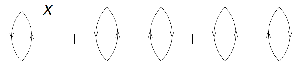
The correponding algebraic expression is \( E_c=\sum_{ia}f^i_a t_i^a +{1\over 4}\sum_{ijab} \langle ij\vert V\vert ab\rangle t_{ij}^{ab} + {1\over 2} \sum_{ijab} \langle ij\vert V\vert ab\rangle t_i^a t_j^b \).
The first algebraic expression is clear. We have one hole line and one
loop, giving it a positive sign. There are no equivalent lines or
vertices, giving it no symmetry factor. The second diagram has two
loops and two hole lines, again leading to a positive sign. We have a
pair of equivalent hole lines and a pair of equivalent particle lines,
each giving a symmetry factor of \( 1/2 \). The third diagram has two
loops and two hole lines, again leading to a positive sign. We have
two indentical vertices (each connecting to a \( T_1 \) in the same way)
and thus a symmetry factor \( 1/2 \).
CCD Approximation
In what follows, we will consider the coupled cluster doubles (CCD)
approximation. This approximation is valid in cases where the system
cannot exhibit any particle-hole excitations (such as nuclear matter
when formulated on a momentum-space grid) or for the pairing model (as
the pairing interactions only excites pairs of particles). In this
case \( t_i^a=0 \) for all \( i, a \), and \( \overline{H}_i^a=0 \). The CCD
approximation is also of some sort of leading order approximation in
the Hartree-Fock basis (as the Hartree-Fock Hamiltonian exhibits no
particle-hole excitations).
Exercise 11: Derive the CCD equations!
Let us consider the matrix element \( \overline{H}_{ij}^{ab} \). Clearly,
it consists of all diagrams (i.e. all combinations of \( T_2 \), and a
single \( F \) or \( V \) that have two incoming hole lines and two outgoing
particle lines. Write down all these diagrams.
Hint.
Start systematically! Consider all combinations of \( F \) and \( V \) diagrams with 0, 1, and 2 cluster amplitudes \( T_2 \).
Answer.
Figure 11: The diagrams for the \( T_2 \) equation, i.e. the matrix elements of \( \overline{H}_{ij}^{ab} \). Taken from Baardsen et al (2013).
The corresponding algebraic expression is
$$
\begin{align*}
\overline{H}_{ij}^{ab} &= \langle ab\vert V\vert ij\rangle + P(ab)\sum_c f_c^bt_{ij}^{ac} - P(ij)\sum_k f_j^k t_{ik}^{ab} \\
&+ {1\over 2} \sum_{cd} \langle ab\vert V\vert cd\rangle t_{ij}^{cd}+ {1\over 2} \sum_{kl} \langle kl\vert V\vert ij\rangle t_{kl}^{ab} + P(ab)P(ij)\sum_{kc} \langle kb\vert V\vert cj \rangle t_{ik}^{ac} \\
&+ {1\over 2} P(ij)P(ab)\sum_{kcld} \langle kl\vert V\vert cd\rangle t_{ik}^{ac}t_{lj}^{db}
+ {1\over 2} P(ij)\sum_{kcld} \langle kl\vert V\vert cd\rangle t_{ik}^{cd}t_{lj}^{ab}\\
&+ {1\over 2} P(ab)\sum_{kcld} \langle kl\vert V\vert cd\rangle t_{kl}^{ac}t_{ij}^{db}
+ {1\over 4} \sum_{kcld} \langle kl\vert V\vert cd\rangle t_{ij}^{cd}t_{kl}^{ab} .
\end{align*}
$$
Let us now turn to the computational cost of a CCD computation.
Exercise 12: Computational scaling of CCD
For each of the diagrams in Fig. 11 write down the
computational cost in terms of the number of occupied \( A \) and the
number of unoccupied \( n_u \) orbitals.
Answer.
The cost is \( A^2 n_u^2 \), \( A^2 n_u^3 \), \( A^3 n_u^2 \),
\( A^2 n_u^4 \), \( A^4 n_u^2 \), \( A^3 n_u^3 \),
\( A^4 n_u^4 \), \( A^4 n_u^4 \),
\( A^4 n_u^4 \), and \( A^4 n_u^4 \) for the respective diagrams.
Note that \( n_u\gg A \) in general. In textbooks, one reads that CCD (and
CCSD) cost only \( A^2n_u^4 \). Our most expensive diagrams, however are
\( A^4n_u^4 \). What is going on?
To understand this puzzle, let us consider the last diagram of
Fig. 11. We break up the computation into two steps,
computing first the intermediate
$$
\begin{align}
\chi_{ij}^{kl}\equiv {1\over 2} \sum_{cd} \langle kl\vert V\vert cd\rangle t_{ij}^{cd}
\label{_auto17}
\end{align}
$$
at a cost of \( A^4n_u^2 \), and then
$$
\begin{align}
{1\over 2} \sum_{kl} \chi_{ij}^{kl} t_{kl}^{ab}
\label{_auto18}
\end{align}
$$
at a cost of \( A^4n_u^2 \). This is affordable. The price to pay is the
storage of the intermediate \( \chi_{ij}^{kl} \), i.e. we traded
memory for computational cycles. This trick is known as
"factorization."
Exercise 13: Factorize the remaining diagrams of the CCD equation
Diagrams 7, 8, and 9 of Fig. 11 also need to be factorized.
Answer.
For diagram number 7, we compute
$$
\begin{align}
\chi_{id}^{al}\equiv\sum_{kc} \langle kl\vert V\vert cd\rangle t_{ik}^{ac}
\label{_auto19}
\end{align}
$$
at a cost of \( A^3 n_u^3 \) and then compute
$$
\begin{align}
{1\over 2} P(ij)P(ab) \sum_{ld} \chi_{id}^{al} t_{lj}^{db}
\label{_auto20}
\end{align}
$$
at the cost of \( A^3 n_u^3 \).
For diagram number 8, we compute
$$
\begin{align}
\chi_{i}^{l}\equiv -{1\over 2} \sum_{kcd} \langle kl\vert V\vert cd\rangle t_{ik}^{cd}
\label{_auto21}
\end{align}
$$
at a cost of \( A^3 n_u^2 \), and then compute
$$
\begin{align}
-P(ij) \sum_l \chi_i^l t_{lj}^{ab}
\label{_auto22}
\end{align}
$$
at the cost of \( A^3 n_u^2 \).
For diagram number 9, we compute
$$
\begin{align}
\chi_d^a\equiv{1\over 2} \sum_{kcl} \langle kl\vert V\vert cd\rangle t_{kl}^{ac}
\label{_auto23}
\end{align}
$$
at a cost of \( A^2 n_u^3 \) and then compute
$$
\begin{align}
P(ab)\sum_d \chi_d^a t_{ij}^{db}
\label{_auto24}
\end{align}
$$
at the cost of \( A^3 n_u^3 \).
We are now ready, to derive the full CCSD equations, i.e. the matrix
elements of \( \overline{H}_i^a \) and \( \overline{H}_{ij}^{ab} \).
Project 14: (Optional) Derive the CCSD equations!
a)
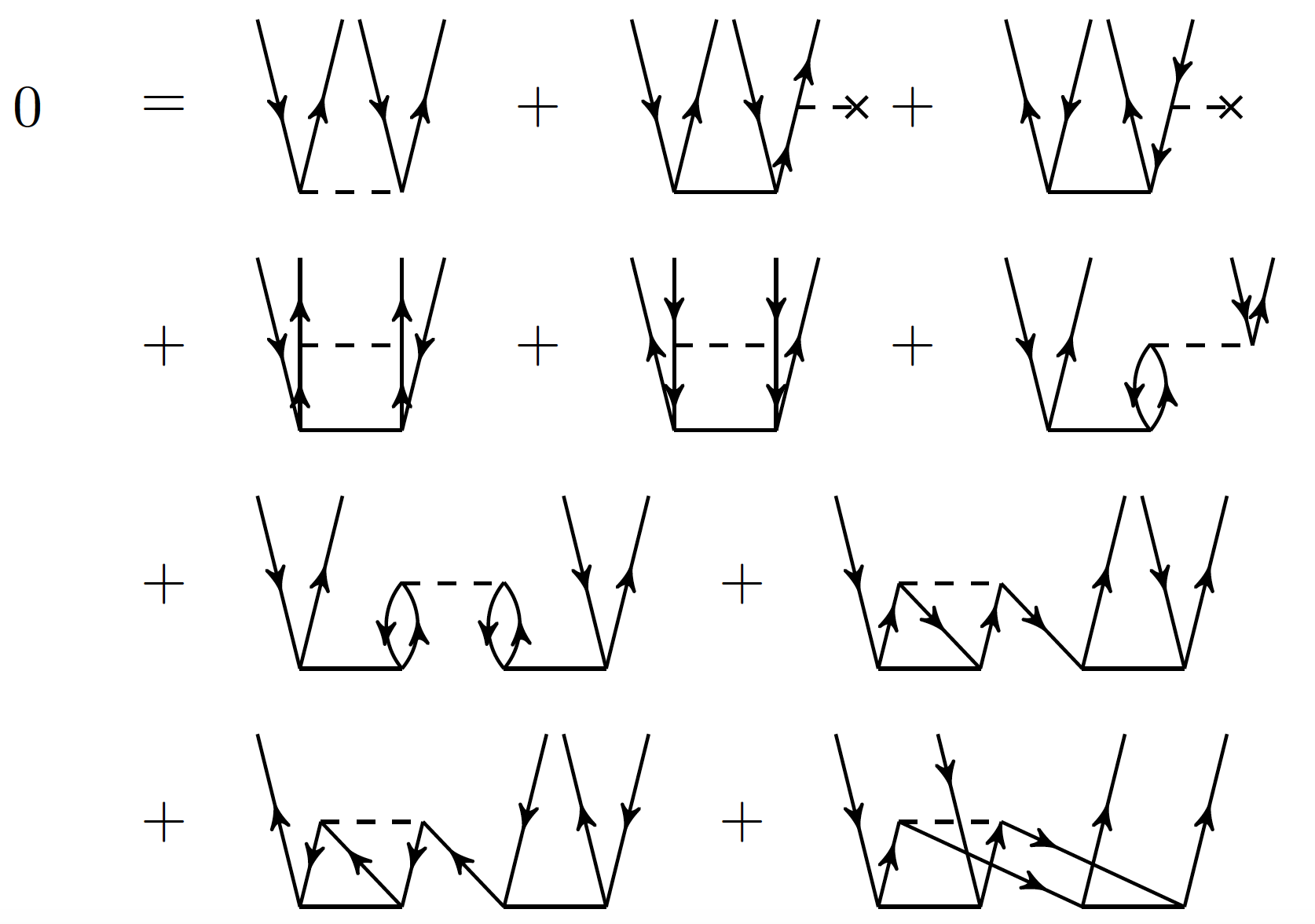
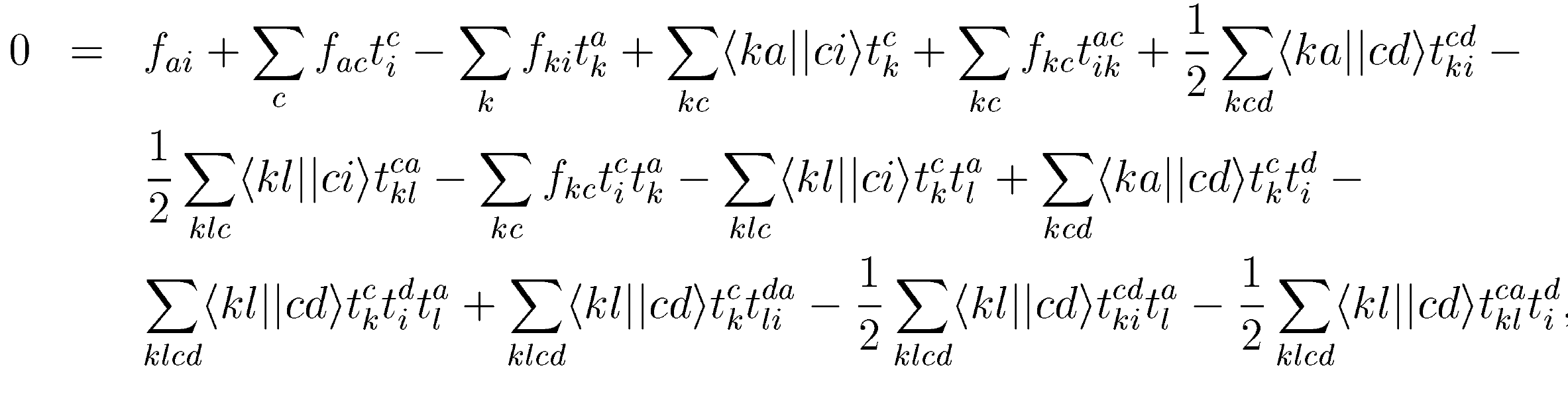
Let us consider the matrix element \( \overline{H}_i^a \) first. Clearly, it consists of all diagrams (i.e. all combinations of \( T_1 \), \( T_2 \), and a single \( F \) or \( V \) that have an incoming hole line and an outgoing particle line. Write down all these diagrams.
Answer.
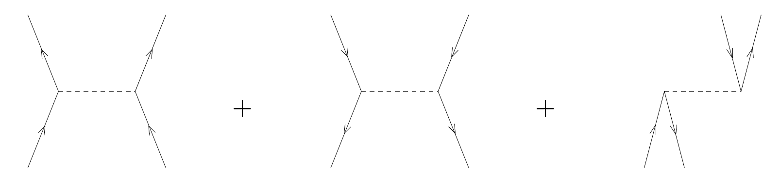
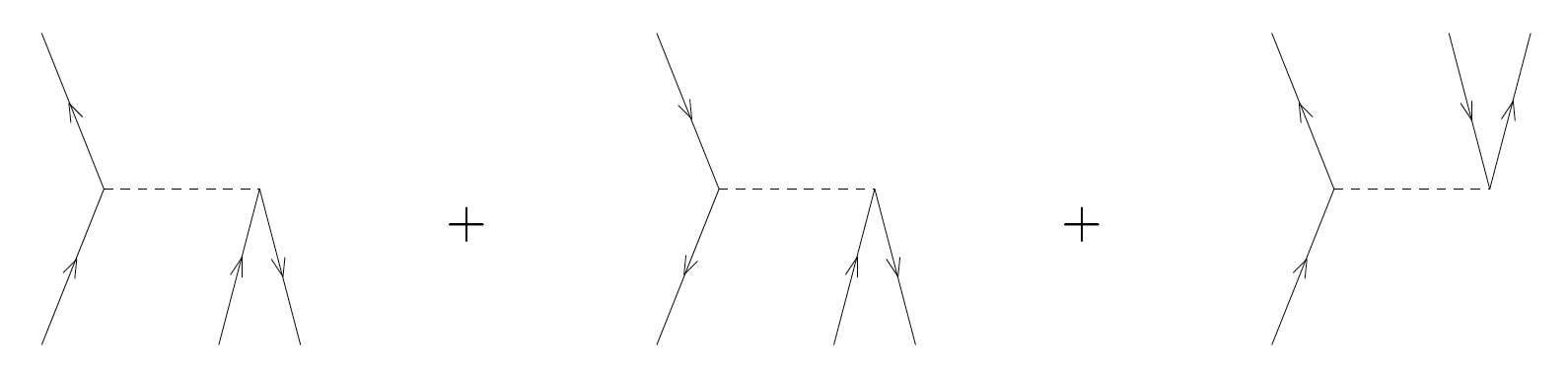
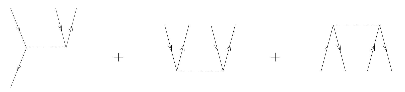
Figure 12: The diagrams for the \( T_1 \) equation, i.e. the matrix elements of \( \overline{H}_i^a \). Taken from Crawford and Schaefer. Here \( \langle pq\vert \vert rs\rangle \equiv \langle pq\vert V\vert rs\rangle \) and \( f_{pq}\equiv f^p_q \).
b)
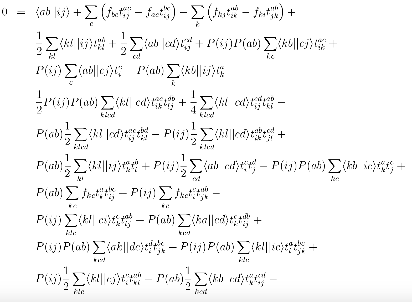
Let us now consider the matrix element \( \overline{H}_{ij}^{ab} \). Clearly, it consists of all diagrams (i.e. all combinations of \( T_1 \), \( T_2 \), and a single \( F \) or \( V \) that have two incoming hole lines and two outgoing particle lines. Write down all these diagrams and corresponding algebraic expressions.
Answer.
Figure 13: The diagrams for the \( T_2 \) equation, i.e. the matrix elements of \( \overline{H}_{ij}^{ab} \). Taken from Crawford and Schaefer. Here \( \langle pq\vert \vert rs\rangle \equiv \langle pq\vert V\vert rs\rangle \), \( f_{pq}\equiv f^p_q \), and \( P(ab) = 1 - (a\leftrightarrow b) \) antisymmetrizes.
We can now turn to the solution of the coupled-cluster equations.
Solving the CCD equations
The CCD equations, depicted in Fig. 11, are nonlinear in the
cluster amplitudes. How do we solve \( \overline{H}_{ij}^{ab}=0 \)? We
subtract \( (f_a^a +f_b^b -f_i^i -f_j^j)t_{ij}^{ab} \) from both sides of
\( \overline{H}_{ij}^{ab}=0 \) (because this term is contained in
\( \overline{H}_{ij}^{ab} \)) and find
$$
\begin{align*}
(f_i^i +f_j^j -f_a^a -f_b^b)t_{ij}^{ab} &= (f_i^i +f_j^j -f_a^a -f_b^b)t_{ij}^{ab} +\overline{H}_{ij}^{ab}
\end{align*}
$$
Dividing by \( (f_i^i +f_j^j -f_a^a -f_b^b) \) yields
$$
\begin{align}
t_{ij}^{ab} &= t_{ij}^{ab} + \frac{\overline{H}_{ij}^{ab}}{f_i^i +f_j^j -f_a^a -f_b^b}
\label{iter}
\end{align}
$$
This equation is of the type \( t=f(t) \), and we solve it by iteration,
i.e. we start with a guess \( t_0 \) and iterate \( t_{n+1}=f(t_n) \), and
hope that this will converge to a solution. We take the perturbative result
$$
\begin{align}
\label{pert}
\left(t_{ij}^{ab}\right)_0 = \frac{\langle ab\vert V\vert ij\rangle}{f_i^i +f_j^j -f_a^a -f_b^b}
\end{align}
$$
as a starting point, compute \( \overline{H}_{ij}^{ab} \), and find a new
\( t_{ij}^{ab} \) from the right-hand side of Eq. \eqref{iter}. We repeat
this process until the amplitudes (or the CCD energy) converge.
CCD for the pairing Hamiltonian
You learned about the pairing Hamiltonian earlier in this
school. Convince yourself that this Hamiltonian does not induce any
1p-1h excitations. Let us solve the CCD equations for this
problem. This consists of the following steps
- Write a function that compute the potential, i.e. it returns a four-indexed array (or tensor). We need \( \langle ab\vert V\vert cd\rangle \), \( \langle ij\vert V\vert kl\rangle \), and \( \langle ab\vert V\vert ij\rangle \). Why is there no \( \langle ab\vert V\vert id\rangle \) or \( \langle ai\vert V\vert jb\rangle \) ?
- Write a function that computes the Fock matrix, i.e. a two-indexed array. We only need \( f_a^b \) and \( f_i^j \). Why?
- Initialize the cluster amplitudes according to Eq. \eqref{pert}, and solve Eq. \eqref{iter} by iteration. The cluster amplitudes \( T_1 \) and \( T_2 \) are two- and four-indexed arrays, respectively.
Please note that the contraction of tensors (i.e. the summation over
common indices in products of tensors) is very user friendly and
elegant in python when numpy.einsum is used.
Project 15: Solve the CCD equations for the pairing problem
The Hamiltonian is
$$
\begin{align}
H = \delta \sum_{p=1}^\Omega (p-1)\left(a^\dagger_{p+}a_{p+} + a^\dagger_{p-}a_{p-}\right)
-{g \over 2} \sum_{p, q=1}^\Omega a^\dagger_{p+}a^\dagger_{p-} a_{q-} a_{q+} .
\label{_auto25}
\end{align}
$$
Check your results and reproduce Fig 8.5 and Table 8.12 from Lecture Notes in Physics 936.
Answer.
Click for IPython notebook for FCI and CCD solutions
## Coupled clusters in CCD approximation
## Implemented for the pairing model of Lecture Notes in Physics 936, Chapter 8.
## Thomas Papenbrock, June 2018

import numpy as np


def init_pairing_v(g,pnum,hnum):
    """
    returns potential matrices of the pairing model in three relevant channels

    param g: strength of the pairing interaction, as in Eq. (8.42)
    param pnum: number of particle states
    param hnum: number of hole states

    return v_pppp, v_pphh, v_hhhh: np.array(pnum,pnum,pnum,pnum),
                                   np.array(pnum,pnum,hnum,hnum),
                                   np.array(hnum,hnum,hnum,hnum),
                                   The interaction as a 4-indexed tensor in three channels.
    """
    v_pppp=np.zeros((pnum,pnum,pnum,pnum))
    v_pphh=np.zeros((pnum,pnum,hnum,hnum))
    v_hhhh=np.zeros((hnum,hnum,hnum,hnum))

    gval=-0.5*g
    for a in range(0,pnum,2):
        for b in range(0,pnum,2):
            v_pppp[a,a+1,b,b+1]=gval
            v_pppp[a+1,a,b,b+1]=-gval
            v_pppp[a,a+1,b+1,b]=-gval
            v_pppp[a+1,a,b+1,b]=gval

    for a in range(0,pnum,2):
        for i in range(0,hnum,2):
            v_pphh[a,a+1,i,i+1]=gval
            v_pphh[a+1,a,i,i+1]=-gval
            v_pphh[a,a+1,i+1,i]=-gval
            v_pphh[a+1,a,i+1,i]=gval

    for j in range(0,hnum,2):
        for i in range(0,hnum,2):
            v_hhhh[j,j+1,i,i+1]=gval
            v_hhhh[j+1,j,i,i+1]=-gval
            v_hhhh[j,j+1,i+1,i]=-gval
            v_hhhh[j+1,j,i+1,i]=gval

    return v_pppp, v_pphh, v_hhhh


def init_pairing_fock(delta,g,pnum,hnum):
    """
    initializes the Fock matrix of the pairing model

    param delta: Single-particle spacing, as in Eq. (8.41)
    param g: pairing strength, as in eq. (8.42)
    param pnum: number of particle states
    param hnum: number of hole states

    return f_pp, f_hh: The Fock matrix in two channels as numpy arrays np.array(pnum,pnum), np.array(hnum,hnum).
    """
# the Fock matrix for the pairing model. No f_ph needed, because we are in Hartree-Fock basis
    deltaval=0.5*delta
    gval=-0.5*g
    f_pp = np.zeros((pnum,pnum))
    f_hh = np.zeros((hnum,hnum))

    for i in range(0,hnum,2):
        f_hh[i  ,i  ] = deltaval*i+gval
        f_hh[i+1,i+1] = deltaval*i+gval

    for a in range(0,pnum,2):
        f_pp[a  ,a  ] = deltaval*(hnum+a)
        f_pp[a+1,a+1] = deltaval*(hnum+a)

    return f_pp, f_hh


def init_t2(v_pphh,f_pp,f_hh):
    """
    Initializes t2 amlitudes as in MBPT2, see first equation on page 345

    param v_pphh: pairing tensor in pphh channel
    param f_pp:   Fock matrix in pp channel
    param f_hh:   Fock matrix in hh channel

    return t2: numpy array in pphh format, 4-indices tensor
    """
    pnum = len(f_pp)
    hnum = len(f_hh)
    t2_new = np.zeros((pnum,pnum,hnum,hnum))
    for i in range(hnum):
        for j in range(hnum):
            for a in range(pnum):
                for b in range(pnum):
                    t2_new[a,b,i,j] = v_pphh[a,b,i,j] / (f_hh[i,i]+f_hh[j,j]-f_pp[a,a]-f_pp[b,b])
    return t2_new


# CCD equations. Note that the "->abij" assignment is redundant, because indices are ordered alphabetically.
# Nevertheless, we retain it for transparency.
def ccd_iter(v_pppp,v_pphh,v_hhhh,f_pp,f_hh,t2):
    """
    Performs one iteration of the CCD equations (8.34), using also intermediates for the nonliniar terms

    param v_pppp: pppp-channel pairing tensor, numpy array
    param v_pphh: pphh-channel pairing tensor, numpy array
    param v_hhhh: hhhh-channel pairing tensor, numpy array
    param f_pp: Fock matrix in pp channel
    param f_hh: Fock matrix in hh channel
    param t2: Initial t2 amplitude, tensor in form of pphh channel

    return t2_new: new t2 amplitude, tensor in form of pphh channel
    """
    pnum = len(f_pp)
    hnum = len(f_hh)
    Hbar_pphh = (  v_pphh
                 + np.einsum('bc,acij->abij',f_pp,t2)
                 - np.einsum('ac,bcij->abij',f_pp,t2)
                 - np.einsum('abik,kj->abij',t2,f_hh)
                 + np.einsum('abjk,ki->abij',t2,f_hh)
                 + 0.5*np.einsum('abcd,cdij->abij',v_pppp,t2)
                 + 0.5*np.einsum('abkl,klij->abij',t2,v_hhhh)
                )

    # hh intermediate, see (8.47)
    chi_hh = 0.5* np.einsum('cdkl,cdjl->kj',v_pphh,t2)

    Hbar_pphh = Hbar_pphh - (  np.einsum('abik,kj->abij',t2,chi_hh)
                             - np.einsum('abik,kj->abji',t2,chi_hh) )

    # pp intermediate, see (8.46)
    chi_pp = -0.5* np.einsum('cdkl,bdkl->cb',v_pphh,t2)

    Hbar_pphh = Hbar_pphh + (  np.einsum('acij,cb->abij',t2,chi_pp)
                             - np.einsum('acij,cb->baij',t2,chi_pp) )

    # hhhh intermediate, see (8.48)
    chi_hhhh = 0.5 * np.einsum('cdkl,cdij->klij',v_pphh,t2)

    Hbar_pphh = Hbar_pphh + 0.5 * np.einsum('abkl,klij->abij',t2,chi_hhhh)

    # phph intermediate, see (8.49)
    chi_phph= + 0.5 * np.einsum('cdkl,dblj->bkcj',v_pphh,t2)


    Hbar_pphh = Hbar_pphh + (  np.einsum('bkcj,acik->abij',chi_phph,t2)
                             - np.einsum('bkcj,acik->baij',chi_phph,t2)
                             - np.einsum('bkcj,acik->abji',chi_phph,t2)
                             + np.einsum('bkcj,acik->baji',chi_phph,t2) )

    t2_new=np.zeros((pnum,pnum,hnum,hnum))
    for i in range(hnum):
        for j in range(hnum):
            for a in range(pnum):
                for b in range(pnum):
                    t2_new[a,b,i,j] = (  t2[a,b,i,j]
                                       + Hbar_pphh[a,b,i,j] / (f_hh[i,i]+f_hh[j,j]-f_pp[a,a]-f_pp[b,b]) )

    return t2_new


def ccd_energy(v_pphh,t2):
    """
    Computes CCD energy. Call as
    energy = ccd_energy(v_pphh,t2)

    param v_pphh: pphh-channel pairing tensor, numpy array
    param t2: t2 amplitude, tensor in form of pphh channel

    return energy: CCD correlation energy
    """
    erg = 0.25*np.einsum('abij,abij',v_pphh,t2)
    return erg

###############################
######## Main Program

# set parameters as for model
pnum = 20 # number of particle states
hnum = 10 # number of hole states
delta = 1.0

g = 0.5

print("parameters")
print("delta =", delta, ", g =", g)


# Initialize pairing matrix elements and Fock matrix
v_pppp, v_pphh, v_hhhh = init_pairing_v(g,pnum,hnum)
f_pp, f_hh = init_pairing_fock(delta,g,pnum,hnum)

# Initialize T2 amplitudes from MBPT2
t2 = init_t2(v_pphh,f_pp,f_hh)
erg = ccd_energy(v_pphh,t2)

# Exact MBPT2 for comparison, see last equation on page 365
exact_mbpt2 = -0.25*g**2*(1.0/(2.0+g) + 2.0/(4.0+g) + 1.0/(6.0+g))
print("MBPT2 energy =", erg, ", compared to exact:", exact_mbpt2)


# iterate CCD equations niter times
niter=200
mix=0.3
erg_old=0.0
eps=1.e-8
for iter in range(niter):
    t2_new = ccd_iter(v_pppp,v_pphh,v_hhhh,f_pp,f_hh,t2)
    erg = ccd_energy(v_pphh,t2_new)
    myeps = abs(erg-erg_old)/abs(erg)
    if myeps < eps: break
    erg_old=erg
    print("iter=", iter, "erg=", erg, "myeps=", myeps)
    t2 = mix*t2_new + (1.0-mix)*t2

print("Energy = ", erg)
Nucleonic Matter
We want to compute nucleonic matter using coupled cluster or IMSRG
methods, and start with considering the relevant symmetries.
Exercise 16: Which symmetries are relevant for nuclear matter?
a)
Enumerate continuous and discrete symmetries of nuclear matter.
Answer.
The symmetries are the same as for nuclei. Continuous symmetries:
translational and rotational invariance. Discrete symmetries: Parity
and time reversal invariance.
b)
What basis should we use to implement these symmetries? Why do we have to make a choice between the two continuous symmetries? Which basis is most convenient and why?
Answer.
Angular momentum and momentum do not commute. Thus, there is no basis
that respects both symmetries simultaneously. If we choose the
spherical basis, we are computing a spherical blob of nuclear matter
and have to contend with surface effects, i.e. with finite size
effects. We also need a partial-wave decomposition of the nuclear
interaction. This approach has been done followed in
["Coupled-cluster studies of infinite nuclear matter, " G. Baardsen,
A. Ekström, G. Hagen, M. Hjorth-Jensen, arXiv:1306.5681, Phys. Rev. C
88, 054312 (2013)]. If we choose a basis of discrete momentum states,
translational invariance can be respected. This also facilitates the
implementetation of modern nuclear interactions (which are often
formulated in momentum space in effective field theories). However, we
have to think about the finite size effects imposed by periodic
boundary conditions (or generalized Bloch waves). This approch was
implemented in ["Coupled-cluster calculations of nucleonic matter,"
G. Hagen, T. Papenbrock, A. Ekström, K. A. Wendt, G. Baardsen,
S. Gandolfi, M. Hjorth-Jensen, C. J. Horowitz, arXiv:1311.2925,
Phys. Rev. C 89, 014319 (2014)].
Basis states
In what follows, we employ a basis made from discrete momentum states,
i.e. those states \( \vert k_x, k_y, k_z\rangle \) in a cubic box of size \( L \) that
exhibit periodic boundary conditions, i.e. \( \psi_k(x+L) =\psi_k(x) \).
Exercise 17: Determine the basis states
What are the discrete values of momenta admissable in \( (k_x, k_y, k_z) \)?
Answer.
In 1D position space \( \psi_k(x) \propto e^{i k x} \) with \( k =
{2\pi n\over L} \) and \( n=0, \pm 1, \pm 2, \ldots \) fulfill \( \psi_k(x+L)
= \psi_k(x) \).
Thus, we use a cubic lattice in momentum space. Note that the
momentum states \( e^{i k x} \) are not invariant under time reversal
(i.e. under \( k\to -k \)), and also do not exhibit good parity (\( x\to
-x \)). The former implies that the Hamiltonian matrix will in general
be complex Hermitian and that the cluster amplitudes will in general
be complex.
Exercise 18: How large should the basis be?
What values should be chosen for the box size \( L \) and for the maximum number \( n_{\rm max} \) , i.e.
for the discrete momenta \( k = {2\pi n\over L} \) and \( n=0, \pm 1,\
\pm 2, \ldots, \pm n_{\rm max} \)?
Answer.
Usually \( n_{\rm max} \) is fixed by computational cost, because we have
\( (2n_{\rm max}+1)^3 \) basis states. We have used \( n_{\rm max}=4 \) or up
to \( n_{\rm max}=6 \) in actual calculations to get converged results.
The maximum momentum must fulfill \( k_{n_{\rm max}}> \Lambda \), where
\( \Lambda \) is the momemtum cutoff of the interaction. This then fixes
\( L \) for a given \( n_{\rm max} \).
Coupled cluster and IMSRG start from a Hartree-Fock reference state,
and we need to think about this next. What are the magic numbers of a
cubic lattice for neutron matter?
Exercise 19: Determine the lowest few magic numbers for a cubic lattice.
Answer.
As the spin-degeneracy is \( g_s=2 \), we have the magic numbers \( g_s N \)
with \( N=1, 7, 19, 27, 33, 57, 66, \ldots \) for neutrons.
Given \( n_{\rm max} \) and \( L \) for the basis parameters, we can choose a
magic neutron number \( N \). Clearly, the density of the system is then
\( \rho=N/L^3 \). This summarizes the requirements for the basis. We
choose \( n_{\rm max} \) as large as possible, i.e. as large as
computationally feasible. Then \( L \) and \( N \) are constrained by the UV
cutoff and density of the system.
Finite size effects
We could also have considered the case of a more generalized boundary
condition, i.e. \( \psi_k(x+L) =e^{i\theta}\psi_k(x) \). Admissable
momenta that fulfill such a boundary condition are \( k_n(\theta) = {2\pi n
+\theta \over L} \). Avering over the "twist" angle \( \theta \) removes
finite size effects, because the discrete momenta are really drawn
form a continuum. In three dimensions, there are three possible twist
angles, and averaging over twist angles implies summing over many
results corresponding to different angles. Thus, the removal of
finite-size effects significantly increases the numerical expense.
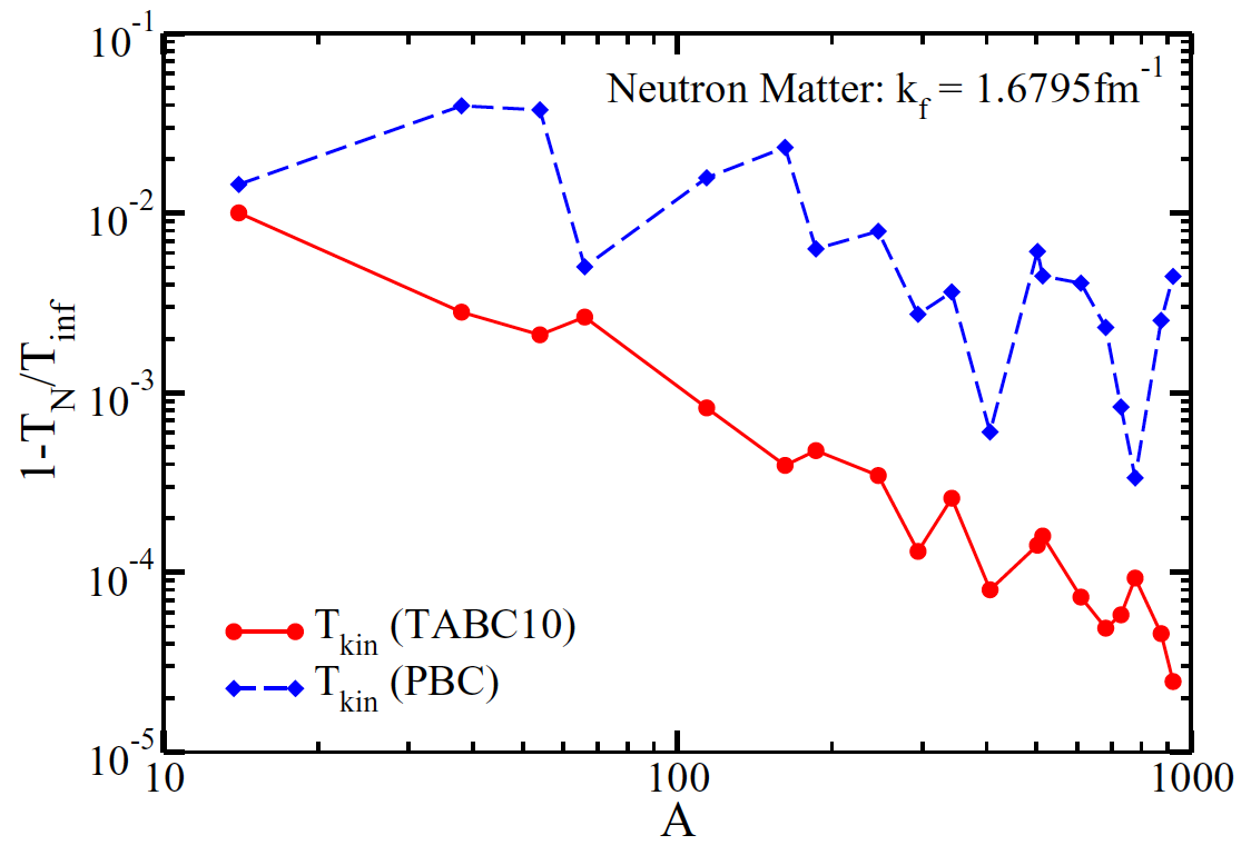
An example
is shown in Figure 14, where we compute the kinetic
energy per particle
$$
\begin{align}
T_N(\theta_x,\theta_y,\theta_z)=g_s\sum_{n_x, n_y, n_z \in N} {\hbar^2 \left( k_{n_x}^2(\theta_x) +k_{n_y}^2(\theta_y) +k_{n_z}^2(\theta_z)\right)\over 2m}
\label{_auto26}
\end{align}
$$
and compare with the infinite result \( T_{\rm inf} = {3\over 10}
{\hbar^2 k_F^2\over m} N \) valid for the free Fermi gas. We clearly see
strong shell effects (blue dashed line) and that averaging over the twist angles
(red full line) very much reduces the shell oscillations. We also note that
the neutron number 66 is quite attractive as it exhibits smaller
finite size effects than other of the accessible magic numbers.
Figure 14: Relative finite-size corrections for the kinetic energy in pure neutron matter at the Fermi momentum \( k_F = 1.6795 {\rm fm}^{-1} \) versus the neutron number A. TABC10 are twist-averaged boundary conditions with 10 Gauss-Legendre points in each spatial direction.
Channel structure of Hamiltonian and cluster amplitudes
Good quantum numbers for the nuclear interaction (i.e. operators that
commute with the Hamiltonian and with each other) are total momentum,
and the number of neutrons and protons, and – for simple interactions
– also the spin (this is really spin, not orbital anular momentum or
total angular momentum, as the latter two do not commute with
momentum). Thus the Hamiltonian (and the cluster amplitudes) will
consist of blocks, one for each set of quantum numbers. We call the
set of quantum numbers that label each such block as a "channel."
As the interaction is block diagonal, a numerically efficient
implementation of nuclear matter has to take advantage of this channel
structure. In fact, neutron matter cannot be computed in a numerically
converged way (i.e. for large enough \( n_{\rm max} \)) if one does not
exploit the channel structure.
The Hamiltonian is of the structure
$$
\begin{align}
\label{HQ}
H = \sum_{\vec{k}, \sigma} \varepsilon_{\vec{k}, \sigma}^{\vec{k}, \sigma} a^\dagger_{\vec{k}, \sigma}a_{\vec{k}, \sigma}
+ \sum_{\vec{Q},\vec{p},\vec{k},\sigma_s} V_{\sigma_1\sigma_2}^{\sigma_3\sigma_4}(\vec{p},\vec{k}) a^\dagger_{\vec{Q/2}+\vec{p}, \sigma_3}a^\dagger_{\vec{Q/2}-\vec{p}, \sigma_4} a_{\vec{Q/2}-\vec{k}, \sigma_2}a_{\vec{Q/2}+\vec{k}, \sigma_1}
\end{align}
$$
with \( \varepsilon_{\vec{k}, \sigma}^{\vec{k}, \sigma} = {k^2\over
2m} \). In Eq. \eqref{HQ} we expressed the single-particle momenta in
terms of center-of-mass momentum \( \vec{Q} \) and relative momenta
\( (\vec{k},\vec{p}) \), i.e. the incoming momenta \( (\vec{k}_1,
\vec{k}_2) \) and outgoing momenta \( (\vec{k}_3, \vec{k}_3) \) are
$$
\begin{align}
\label{CoM}
\vec{k}_1 &= \vec{Q}/2 +\vec{k} ,\\
\vec{k}_2 &= \vec{Q}/2 -\vec{k} ,
\label{_auto27}\\
\vec{k}_3 &= \vec{Q}/2 +\vec{p} ,
\label{_auto28}\\
\vec{k}_4 &= \vec{Q}/2 -\vec{p} .
\label{_auto29}
\end{align}
$$
The conservation of momentum is obvious in the two-body interaction as
both the annihilation operators and the creation operators depend on
the same center-of-mass momentum \( \vec{Q} \). We note that the two-body
interaction \( V \) depends only on the relative momenta
\( (\vec{k},\vec{p}) \) but not on the center-of-mass momentum. We also
note that a local interaction (i.e. an interaction that is
multiplicative in position space) depends only on the momentum
transfer \( \vec{k}-\vec{p} \). The spin projections \( \pm 1/2 \) are denoted
as \( \sigma \).
Thus, the \( T_2 \) operator is
$$
\begin{align}
\label{t2Q}
T_2 = {1\over 4} \sum_{\vec{Q},\vec{p},\vec{k},\sigma_s} t_{\sigma_1\sigma_2}^{\sigma_3\sigma_4}(Q; \vec{p},\vec{k}) a^\dagger_{\vec{Q/2}+\vec{p}, \sigma_3}a^\dagger_{\vec{Q/2}-\vec{p}, \sigma_4} a_{\vec{Q/2}-\vec{k}, \sigma_2}a_{\vec{Q/2}+\vec{k}, \sigma_1} .
\end{align}
$$
We note that the amplitude \( t_{\sigma_1\sigma_2}^{\sigma_3\sigma_4}(Q;
\vec{p},\vec{k}) \) depends on the center-of-mass momentum \( \vec{Q} \), in
contrast to the potential matrix element
\( V_{\sigma_1\sigma_2}^{\sigma_3\sigma_4}(\vec{p},\vec{k}) \).
In the expressions \eqref{HQ} and \eqref{t2Q} we supressed that
\( \sigma_1+\sigma_2 = \sigma_3+\sigma_4 \). So, a channel is defined by
\( \vec{Q} \) and total spin projection \( \sigma_1+\sigma_2 \).
Because of this channel structure, the simple solution we implemented
for the pairing problem cannot be really re-used when computing
neutron matter. Let us take a look at the Minnesota potential
$$
\begin{align}
V(r) = \left( V_R(r) + {1\over 2}(1+P_{12}^\sigma)V_T(r) + {1\over 2}(1-P_{12}^\sigma)V_S(r)\right) {1\over 2}(1-P_{12}^\sigma P_{12}^\tau).
\label{_auto30}
\end{align}
$$
Here,
$$
\begin{align}
P^\sigma_{12}&= {1\over 2}(1+\vec{\sigma}_1\cdot\vec{\sigma}_2) , \nonumber\\
P^\tau_{12} &= {1\over 2}(1+\vec{\tau}_1\cdot\vec{\tau}_2)
\label{_auto31}
\end{align}
$$
are spin and isospin exchange operators, respectively, and
\( \vec{\sigma} \) and \( \vec{\tau} \) are vectors of Pauli matrices in spin
and isospin space, respectively. Thus,
$$
\begin{align}
{1\over 2}(1-P_{12}^\sigma P_{12}^\tau) & = \vert
S_{12}=0, T_{12}=1\rangle\langle S_{12}=0,T_{12}=1\vert + \vert
S_{12}=1, T_{12}=0\rangle\langle S_{12}=1,T_{12}=0\vert
\label{_auto32}
\end{align}
$$
projects onto two-particle spin-isospin states as indicated, while
$$
\begin{align}
{1\over 2}(1-P_{12}^\sigma) & = \vert
S_{12}=0\rangle\langle S_{12}=0\vert ,
\label{_auto33}\\ {1\over 2}(1+P_{12}^\sigma)
& = \vert S_{12}=1\rangle\langle S_{12}=1\vert
\label{_auto34}
\end{align}
$$
project onto spin singlet and spin triplet combinations,
respectively. For neutron matter, two-neutron states have isospin
\( T_{12}=1 \), and the Minnesota potential has no triplet term \( V_T \).
For the spin-exchange operator (and spins \( s_1, s_2=\pm 1/2 \)), we have
\( P_{12}^\sigma\vert s_1s_2\rangle= \vert s_2s_1\rangle \). For neutron
matter, \( P_{12}^\tau=1 \), because the states are symmetric under exchange of
isospin. Thus, the Minnesota potential simplifies significantly for
neutron matter as \( V_T \) does not contribute.
We note that the spin operator has matrix elements
$$
\begin{align}
\langle s_1' s_2'\vert {1\over 2}(1-P_{12}^{\sigma})\vert s_1 s_2\rangle
= {1\over 2} \left(
\delta_{s_1}^{s_1'}\delta_{s_2}^{s_2'}
-\delta_{s_1}^{s_2'}\delta_{s_2}^{s_1'}\right) .
\label{_auto35}
\end{align}
$$
The radial functions are
$$
\begin{align}
V_R(r) &=V_R e^{-\kappa_R r^2} ,
\label{_auto36}\\
V_S(r) &=V_S e^{-\kappa_S r^2} ,
\label{_auto37}\\
V_T(r) &=V_T e^{-\kappa_T r^2} ,
\label{_auto38}\\
\label{_auto39}
\end{align}
$$
and the parameters are as follows
| \( \alpha \) | \( V_\alpha \) | \( \kappa_\alpha \) |
| \( R \) | +200 MeV | 1.487 fm \( ^{-2} \) |
| \( S \) | -91.85 MeV | 0.465 fm \( ^{-2} \) |
| \( T \) | -178 MeV | 0.639 fm \( ^{-2} \) |
Note that \( \kappa_\alpha^{1/2} \) sets the momentum scale of the
Minnesota potential. We see that we deal with a short-ranged repulsive
core (the \( V_R \) term) and longer ranged attractive terms in the
singlet (the term \( V_S \)) and triplet (the term \( V_T \)) channels.
A Fourier transform (in the finite cube of length \( L \)) yields the momentum-space form of the potential
$$
\begin{align}
\langle k_p k_q \vert V_\alpha\vert k_r k_s \rangle = {V_\alpha\over L^3} \left({\pi\over\kappa_\alpha}\right)^{3/2}
e^{- {q^2 \over 4\kappa_\alpha}} \delta_{k_p+k_q}^{k_r+k_s} .
\label{_auto40}
\end{align}
$$
Here, \( q\equiv {1\over 2}(k_p-k_q-k_r+k_s) \) is the momentum transfer,
and the momentum conservation \( k_p+k_q=k_r+k_s \) is explicit.
As we are dealing only with neutrons, the potential matrix elements
(including spin) are for \( \alpha = R, S \)
$$
\begin{align}
\label{ME_of_V}
\langle k_p s_p k_q s_q\vert V_\alpha\vert k_r s_r k_s s_s\rangle &= \langle k_p k_q \vert V_\alpha\vert k_r k_s \rangle
{1\over 2}\left(\delta_{s_p}^{s_r}\delta_{s_q}^{s_s} - \delta_{s_p}^{s_s}\delta_{s_q}^{s_r}\right) ,
\end{align}
$$
and it is understood that there is no contribution from \( V_T \). Please note that the matrix elements \eqref{ME_of_V} are not yet antisymmetric under exchange, but \( \langle k_p s_p k_q s_q\vert V_\alpha\vert k_r s_r k_s s_s\rangle -
\langle k_p s_p k_q s_q\vert V_\alpha\vert k_s s_s k_r s_r\rangle \) is.
Example: Channel structure and its usage
We have single-particle states with momentum and spin, namely
$$
\begin{align}
\vert r\rangle \equiv \vert k_r s_r\rangle .
\label{_auto41}
\end{align}
$$
Naively, two-body states are then
$$
\begin{align}
\vert r s \rangle \equiv \vert k_r s_r k_s s_s\rangle ,
\label{_auto42}
\end{align}
$$
but using the center-of-mass transformation \eqref{CoM} we can rewrite
$$
\begin{align}
\vert r s \rangle \equiv \vert P_{rs} k_{rs} s_r s_s\rangle ,
\label{_auto43}
\end{align}
$$
where \( P_{rs} = k_r +k_s \) is the total momentum and
\( k_{rs}=(k_r-k_s)/2 \) is the relative momentum. This representation of
two-body states is well adapated to our problem, because the
interaction and the \( T_2 \) amplitudes preserve the total momentum.
Thus, we store the cluster amplitudes \( t_{ij}^{ab} \) as matrices
$$
\begin{align}
t_{ij}^{ab} \to \left[t(P_{ij})\right]_{\vert k_{ij} s_i s_j\rangle}^{\vert k_{ab} s_a s_b\rangle}
\equiv t_{\vert P_{ij} k_{ij} s_i s_j\rangle}^{\vert P_{ij} k_{ab} s_a s_b\rangle} ,
\label{_auto44}
\end{align}
$$
and the conservation of total momentum is explicit.
Likewise, the pppp, pphh, and hhhh parts of the interaction can be written in this form, namely
$$
\begin{align}
V_{cd}^{ab} &\to \left[V(P_{ab})\right]_{\vert k_{cd} s_c s_d\rangle}^{\vert k_{ab} s_a s_b\rangle}
\equiv V_{\vert P_{ab} k_{cd} s_c s_d\rangle}^{\vert P_{ab} k_{ab} s_a s_b\rangle} ,
\label{_auto45}\\
V_{ij}^{ab} &\to \left[V(P_{ij})\right]_{\vert k_{ij} s_i s_j\rangle}^{\vert k_{ab} s_a s_b\rangle}
\equiv V_{\vert P_{ij} k_{ij} s_i s_j\rangle}^{\vert P_{ij} k_{ab} s_a s_b\rangle} ,
\label{_auto46}\\
V_{ij}^{kl} &\to \left[V(P_{ij})\right]_{\vert k_{ij} s_i s_j\rangle}^{\vert k_{kl} s_k s_l\rangle}
\equiv V_{\vert P_{ij} k_{ij} s_i s_j\rangle}^{\vert P_{ij} k_{kl} s_k s_l\rangle} ,
\label{_auto47}
\end{align}
$$
and we also have
$$
\begin{align}
\overline{H}_{ij}^{ab} \to \left[\overline{H}(P_{ij})\right]_{\vert k_{ij} s_i s_j\rangle}^{\vert k_{ab} s_a s_b\rangle}
\equiv \overline{H}_{\vert P_{ij} k_{ij} s_i s_j\rangle}^{\vert P_{ij} k_{ab} s_a s_b\rangle} ,
\label{_auto48}
\end{align}
$$
Using these objects, diagrams (1), (4), and (5) of Figure
11 can be done for each block of momentum \( P_{ij} \) as a
copy and matrix-matrix multiplications, respectively
$$
\begin{align}
\left[\overline{H}(P_{ij})\right]_{\vert k_{ij} s_i s_j\rangle}^{\vert k_{ab} s_a s_b\rangle} &=
\left[V(P_{ij})\right]_{\vert k_{ij} s_i s_j\rangle}^{\vert k_{ab} s_a s_b\rangle}
\label{_auto49}\\
&+ {1\over 2} \sum_{\vert k_{kl} s_k s_l\rangle}
\left[t(P_{ij})\right]_{\vert k_{kl} s_k s_l\rangle}^{\vert k_{ab} s_a s_b\rangle}
\left[V(P_{ij})\right]_{\vert k_{ij} s_i s_j\rangle}^{\vert k_{kl} s_k s_l\rangle}
\label{_auto50}\\
&+ {1\over 2} \sum_{\vert k_{cd} s_c s_d\rangle}
\left[V(P_{ij})\right]_{\vert k_{cd} s_c s_d\rangle}^{\vert k_{ab} s_a s_b\rangle}
\left[t(P_{ij})\right]_{\vert k_{ij} s_i s_j\rangle}^{\vert k_{cd} s_c s_d\rangle} .
\label{_auto51}
\end{align}
$$
Similarly, the CCD correlation energy results from
$$
\begin{align}
E_c = {1\over 4} \sum_{P_{ij}} \sum_{\vert k_{ij} s_i s_j\rangle}\sum_{\vert k_{ab} s_a s_b\rangle }
\left[t(P_{ij})\right]_{\vert k_{ij} s_i s_j\rangle}^{\vert k_{ab} s_a s_b\rangle}
\left[V(P_{ij})\right]_{\vert k_{ij} s_i s_j\rangle}^{\vert k_{ab} s_a s_b\rangle}
\label{_auto52}
\end{align}
$$
These efficiences cannot be used for the sixth diagram of Figure
11. One could either change to a ph formulation, noting that
\( k_a-k_i = k_k -k_c \) is also a preserved quantity in \( t_{ik}^{ac} \) and
that \( k_k-k_c = k_j-k_b \) is preserved in \( V_{cj}^{kb} \). Thus
\( \sum_{kc} t_{ik}^{ac}V_{cj}^{kb} \) has a conserved quantity \( k_k-k_c \)
in the loop, and we can again use matrix-matrix multiplications for
this diagram. This requires us to store the \( T_2 \) amplitude in a phhp
and in the usual pphh formulation. Alternatively, we could simply code
this diagram with the loops over single-particle states. If this seems
too tedious, one can also limit CCD to the first five diagrams in
Figure 11 (these are the pp and hh ladders), which gives a
good description for neutron matter, see the comparison between this
and full CCD in ["Coupled-cluster calculations of nucleonic matter,"
G. Hagen, T. Papenbrock, A. Ekström, K. A. Wendt, G. Baardsen,
S. Gandolfi, M. Hjorth-Jensen, C. J. Horowitz, arXiv:1311.2925,
Phys. Rev. C 89, 014319 (2014)].
The steps towards the solution of the CCD equations for neutron matter are as follows
- For a given density and UV cutoff, set up the lattice, i.e. determine the single-particle basis.
- Determine the channels allowed by the (Minnesota) interaction, i.e. sets of two-body states that are connected by the interaction.
- Exploit this channel structure when computing the diagrams.
- Solve the coupled-cluster equations. Here we start first with the pp and hh ladders, i.e. using only the first five diagrams of Figure 11.
Exercise 20: Write a CCD code for neutron matter, focusing first on ladder approximation, i.e. including the first five diagrams in Figure 11.
Answer.
Click for IPython notebook
import numpy as np

##############################################################
# CCD Program for neutron matter with the Minnesota potential.
#
# Thomas Papenbrock, July/August 2018
#
# License: Free Software following Version 3 of GNU General Public License,
# see https://www.gnu.org/licenses/gpl.html
#######


##########################
# Class for neutron matter
#######

class MomSpaceBasis:
    """
    momentum-space basis class
    The constructor has the form

    MomSpaceBasis(Nmax,kmax)

    param Nmax: Number of lattice points in positive kx-direction
    param kmax: Highest lattice momentum (in 1/fm)

    return: MomSpaceBasis as a single-partcle basis.
    attributes of MomSpaceBasis are

    dk : lattice spacing in 1/fm
    Lbox : linear dimension (in fm) of cubic box
    nvec : lattice vectors (integers)
    kvec : lattice momentum vectors (floats, in 1/fm)
    ngrid : total number of lattice points
    """
    def __init__(self,Nmax,kmax,ordered=True):
        """
        the constructor

        Generates a cubic lattice in momentum space
        param Nmax: Number of lattice points in positive kx-direction
        param kmax: Highest lattice momentum (in 1/fm)
        param ordered: Optional parameter, True by default, will order lattice points by kinetic energy

        return MomSpaceBasis
        """
        self.Nmax = Nmax
        self.dim = 0
        self.ngrid = 0
        self._kvec=[]
        self._nvec=[]

        dk = kmax / Nmax
        self.dk = dk
        self.Lbox = 2.0*np.pi/dk

        nx=[]
        nvec=[]
        for i in range(-Nmax,Nmax+1):
            self.dim=self.dim+1
            nx.append(i)

        #print('nx=',nx)

        for i in nx:
            for j in nx:
                for k in nx:
                    nvec.append(np.array([i,j,k], dtype=int))

        #print('nvec=',nvec)
        self.ngrid=len(nvec)

        if ordered:
            #print("ordered")
            norm=np.zeros(self.ngrid,dtype=int)
            for i, vec in enumerate(nvec):
                npvec=np.array(vec,dtype=int)
                norm[i]=np.dot(npvec,npvec)
               # print(i, vec, norm[i])

            index=np.argsort(norm)
            #print(index)
            self._nvec=[]
            for i, ind in enumerate(index):
                #print(i, ind, nvec[ind])
                self._nvec.append(nvec[ind])

        else:
            self._nvec=nvec  # a list

        self._kvec = np.array(self._nvec)*dk # a numpy array


    def kvec(self,indx=-1):
        """
        MomSpaceBasis.kvec(i) returns ith momentum vector
        MomSpaceBasis.kvec() returns all momentum vectors

        param indx: index of k-vector to be returned, optional
        return 3-vector (if index non-negative), or all vectors if no index specified
        """
        if indx == -1:
            return self._kvec
        else:
            return self._kvec[indx]

    def nvec(self,indx=-1):
        """
        MomSpaceBasis.nvec(i) returns ith lattice vector
        MomSpaceBasis.nvec() returns all lattice vectors

        param indx: index of lattice vector to be returned, optional
        return 3-vector (if index non-negative), or all lattice vectors if no index specified
        """
        if indx == -1:
            return self._nvec
        else:
            return self._nvec[indx]

    def dens(self,num):
        """
        returns density of system if num particles are present
        param num: int, number of particles
        return dens: float
        """
        return num/(self.Lbox)**3

    def update(self,dk):
        """
        Uses dk as new lattice spacing and rescales existing lattice
        param dk: in 1/fm lattice spacing in momentum space
        """
        self.Lbox=2.0*np.pi/dk
        self._kvec = np.array(self._nvec)*dk

    def __len__(self):
        """
        overloading of the 'len' function
        """
        return self.ngrid


############
# useful functions

def magic_numbers(basis):
    """
    param basis: MomSpaceBasis object
    return magic: array of magic numbers
    """
    nvecs = basis.nvec()
    vec=np.array(nvecs[0],dtype=int)
    norm = np.dot(vec,vec)
    magic=[]
    for i in range(1,len(nvecs)):
        vec=np.array(nvecs[i],dtype=int)
        norm2 = np.dot(vec,vec)
        if norm2 > norm:
            magic.append(2*i)
            norm=norm2
    return magic


def get_dk(rho,Num):
    """
    param rho: desired density
    param Num: magic number of particles
    return dk: grid spacing in momentum space (in 1/fm)
    """
    Lbox = (Num/rho)**(1.0/3.0)
    dk = 2.0*np.pi/Lbox
    return dk

def spbasis_from_MomSpaceBasis(lattice_vecs,st_degen):
    """
    converts a lattice to a single particle basis for spin-isospin degeneracy st_degen
    param lattice_vecs: list of lattice vectors for 1st particle
    param st_degen: spin-isospin degeneracy
    return: basis as a list of momenta
    """
    if st_degen != 2: # for now only neutron matter
        print("Unexpected parameter st_degen")
        return lattice_vecs

    basis=[]
    for vec in lattice_vecs:
        for st in range(st_degen):
            basis.append(np.array(vec,dtype=int))

    return basis


#########################################################
# Functions for comparisons with infinite free Fermi gas

def kF_from_density(rho,st_degen=2):
    """
    Computes Fermi momentum for given density and spin/isospin degeneracy.

    param rho: density in inverse fm cubed
    param st_degen: spin-isospin degeneracy; default 2
    return: Fermi momentum in inverse fm
    """
    res = (6.0*(np.pi)**2*rho/st_degen)**(1.0/3.0)
    return res

def EnergyDensity_FermiGas(kF,st_degen=2):
    """
    Computes energy density of free Fermi gas at Fermi momentum and spin/isospin degeneracy
    param kF: Fermi momentum in inverse fm
    param st_degen: spin-isospin degeneracy; default 2
    return: Energy density in MeV/fm**3
    """
    pvec = np.array([kF,0.0,0.0])
    erg = (st_degen*kF**3/(10.0*np.pi**2)) * Tkin(pvec)
    return erg


########################################################################################
# Functions for CCD of neutron matter
# Implementation uses only pp and hh ladders
#
########################################################################################


from numba import jit
# compile a few functions to gain speed; should probably done in Fortran or C++,
# and called from Python

@jit(nopython=True)
def minnesota_nn(p_out,s1_out,s2_out,p_in,s1_in,s2_in,Lbox):
    """
    The Minnesota potential between two neutrons, not yet anti-symmetrized
    param p_out: relative out momentum
    param p_in : relative in momentum
    param s1_out, s2_out: spin projections of out particles 1 and 2
    param s1_in, s2_in  : spin projections of in particles 1 and 2
    Lbox : size of momentum box
    return: value of potential in MeV; not anti-symmetrized!
    """
    # parameters. VT is not active between two neutrons (no triplet)
    VR = 200.0
    VS = -91.85  # sign typo in Lecture Notes Physics 936, Chap. 8
    kappaR = 1.487
    kappaS = 0.465

    qvec=p_out-p_in
    q2=np.dot(qvec,qvec)

    s1_i =spin2spinor(s1_in)
    s2_i =spin2spinor(s2_in)
    s1_o =spin2spinor(s1_out)
    s2_o =spin2spinor(s2_out)

    spin_part = 0.5 * ( np.dot(s1_i,s1_o)*np.dot(s2_i,s2_o)
                       -np.dot(s1_i,s2_o)*np.dot(s2_i,s1_o) )


    pot = spin_part * (  VR*np.exp(-0.25*q2/kappaR) / (Lbox*np.sqrt(kappaR))**3
                       + VS*np.exp(-0.25*q2/kappaS) / (Lbox*np.sqrt(kappaS))**3 )

    pot = pot*(np.sqrt(np.pi))**3


    return pot

@jit
def spin_of_index(i):
    """
    Even indices of the lattive have spin up, odds have spin down
    param i: index of sp_basis
    return: spin as +/- 1
    """
    spin = 1-2*np.remainder(i,2)
    return spin

@jit
def spin2spinor(s):
    """
    Makes a two-component spinor of an integer s
    param s: spin = +/- 1
    return: two-component numpy array [1,0] for up and [0,1] for down
    """
    up  =np.array([1.0,0.0])
    down=np.array([0.0,1.0])
    if s == 1:
        return up
    else:
        return down

@jit
def Tkin(pvec):
    """
    Kinetic energy for a momentum vector
    param pvec: 3-component numpy array in inverse fm
    return: kinetic energy of that momentum in MeV
    """
    nucleon_mass = 938.92
    hbarc = 197.33
# More precise numbers for neutron mass and hbar follow.
# For N=14, this yields E_HF = 10.3337 MeV per nucleon in HF. Benchmarked with Ragnar Stroberg.
#     nucleon_mass = 939.56563
#     hbarc = 197.3269718
    p2 = np.dot(pvec,pvec)
    res = 0.5*hbarc**2*p2/nucleon_mass
    return res

@jit
def compute_total_Tkin(Nocc,sp_basis,dk):
    """
    Computes total kinetic energy of reference state
    param Nocc, sp_basis, dk: particle number, integer s.p. lattice, delta k
    return: total kinetic energy
    """
    erg=0.0
    for i in range(Nocc):
        mom_vec = sp_basis[i]
        vec=np.array(mom_vec)*dk
        erg=erg+Tkin(vec)

    return erg


@jit
def Fock(pvec,s,sp_basis,Nocc,dk,Lbox):
    """
    Fock matrix of momentum pvec in hh space
    param pvec: 3-component numpy array in inverse fm
    param s: spin as +/- 1 of state
    param_sp_basis, Nocc, dk, Lbox : parameters of s.p. basis and system

    return: Fock matrix element = kinetic energy of that momentum in MeV
    """
    res = Tkin(pvec)

    dum=0.0
    for i in range(Nocc):
        vec=sp_basis[i]*dk
        si=spin_of_index(i)
        p_in = 0.5*(vec-pvec)
        p_out= p_in
        dum = dum + ( minnesota_nn(p_out,s,si, p_in, s,si,Lbox)
                     -minnesota_nn(p_out,s,si,-p_in,si, s,Lbox) )  #antisymmetrized Minnesota

    res = res+dum
    return res

def compute_E_HF_simple(Nocc,sp_basis,dk):
    """
    Computes HF energy of reference state
    param Nocc, sp_basis, dk: particle number, integer s.p. lattice, delta k
    return: total HF energy
    """
    erg=compute_total_Tkin(Nocc,sp_basis,dk)

    pot=0.0
    for i in range(Nocc):
        momi=sp_basis[i]*dk
        si = spin_of_index(i)
        for j in range(Nocc):
            momj=sp_basis[j]*dk
            sj = spin_of_index(j)
            p_rel = 0.5*(momi-momj)
            pot = pot + 0.5* (  minnesota_nn(p_rel,si,sj, p_rel,si,sj,Lbox)
                                - minnesota_nn(p_rel,si,sj,-p_rel,sj,si,Lbox) )

    erg = erg+pot
    return erg


def get_channels(sp_basis,start1,end1,start2,end2,identical,other_channels=None):
    """
    Returns channels for coupled cluster based on Minnesota potential
    param sp_Basis: A single-particle basis
    param start1: index to start for particle 1
    param end1: index to end for particle 1
    param start2: index to start for particle 2
    param end2: index to end for particle 2
    param identical: True for hh or pp, False for hp
    param other_channels: list of other channels to compare with
    return: channels, p_rel, t2amp. channels is a list of p12, where p12 is a momentum vector;
            p_rel is a nested list with relative momenta and spins for each channel
    """
    channel=[]
    p_rel=[]
    for i, mom_vecs1 in enumerate(sp_basis[start1:end1]):
        #vec1=np.array(mom_vecs1,dtype=int)
        vec1=mom_vecs1
        spin1=spin_of_index(i)

        for j, mom_vecs2 in enumerate(sp_basis[start2:end2]):
            if identical and i==j: continue  #Fortran cycle
            #vec2=np.array(mom_vecs2,dtype=int)
            vec2=mom_vecs2
            spin2=spin_of_index(j)

            p12 = vec1+vec2
            prel= vec1-vec2
            spins=np.array([spin1,spin2],dtype=int)
            ps=[prel,spins]

            new=True
            needed=True
            if other_channels is not None: #check whether we need this channel
                needed=False
                for chan_o in other_channels:
                    if (chan_o==p12).all():
                        needed=True
                        break
            if needed: #check whether this channel exists already
                for ipos, chan in enumerate(channel):
                    if (chan==p12).all():
                        new=False
                        break

            if needed and new:
                channel.append(p12)
                p_rel.append([ps])

            if needed and not new:
                p_rel[ipos].append(ps)

    return channel, p_rel


def setup_T2_amplitudes(sp_basis,NN,st_degen):
    """
    returns the t2 amplitudes and t2 channels
    param sp_basis: a sp_basis
    param NN: neutron number
    param st_degen: 2 for the moment, spin-isospin degeneracy
    return: hh_channels, pp_channels, p_rel_hh, p_rel_pp, t2amp
            these are the hh and pp channels of T2, lists of the relative momenta,
            and t2amps as a list of numpy arrays set to zero
    """
    num_states = len(sp_basis)

    hh_channels, p_rel_hh = get_channels(sp_basis,0,NN,0,NN,True)
    print('hh channels=', len(hh_channels))

    pp_channels, p_rel_pp = get_channels(sp_basis,NN,num_states,NN,num_states,True,hh_channels)
    print('pp channels=', len(pp_channels))

    if len(pp_channels) != len(hh_channels): print('pp and hh channels do not match')


    ordered_pp_channel=[]
    ordered_p_rel_pp=[]
    for i, chanhh in enumerate(hh_channels):
        for j, chanpp in enumerate(pp_channels):
            if (chanpp==chanhh).all():
                ordered_pp_channel.append(chanpp)
                ordered_p_rel_pp.append(p_rel_pp[j])
                break

    pp_channels = ordered_pp_channel
    p_rel_pp = ordered_p_rel_pp

    # set t2 amplitudes to zero in each channel
    t2amp = fill_pot(Lbox, dk, pp_channels, hh_channels, p_rel_pp, p_rel_hh, True)

    return hh_channels, pp_channels, p_rel_hh, p_rel_pp, t2amp

def fill_pot(Lbox, dk, channels_out, channels_in, p_rel_out, p_rel_in, T2amp=False):
    """
    Fills lists of matrices such as Vhhhh, Vpphh, Vpppp, t2_pphh
    param Lbox: Lbox
    param dk: dk
    param channels_out, channels_in: the channels we have
    param p_rel_out, p_rel_in: the list of [prel, [s1,s2]]
    param T2amp=False: Set to True if t2_pphh needs to be computed
    return: The object of desire as a list of numpy matrices.
            Contain matrix elements for potentials, zeros if T2amp=True is requested.
    """
    Vpot=[]
    for i, chan_in in enumerate(channels_in):
        dim_in = len(p_rel_in[i])
        dim_out= len(p_rel_out[i])
        Vpot_chan=np.zeros((dim_out,dim_in))
        if not T2amp:
            for ii, ps_i in enumerate(p_rel_in[i]):
                [pii, [s1, s2]] = ps_i
                pii = pii*dk*0.5
                for jj, ps_j in enumerate(p_rel_out[i]):
                    if dim_in == dim_out and jj > ii: continue
                    [pjj, [ss1, ss2]] = ps_j
                    pjj = pjj*dk*0.5
                    Vpot_chan[jj,ii] = ( minnesota_nn( pjj,ss1,ss2, pii,s1,s2,Lbox)
                                        -minnesota_nn(-pjj,ss2,ss1, pii,s1,s2,Lbox) )
                    if dim_in == dim_out : Vpot_chan[ii,jj] = Vpot_chan[jj,ii]

        Vpot.append(Vpot_chan)
    return Vpot


def init_V(Lbox, dk, hhchannels, ppchannels, p_relhh, p_relpp,zeros=False):
    """
    Sets up Vhhhh, Vpphh, and Vpppp.

    return: Vhhhh, Vpphh, Vpppp as a lists of numpy arrays
    """
    Vhhhh = fill_pot(Lbox, dk, hhchannels, hhchannels, p_relhh, p_relhh,zeros)
    Vpphh = fill_pot(Lbox, dk, ppchannels, hhchannels, p_relpp, p_relhh,zeros)
    Vpppp = fill_pot(Lbox, dk, ppchannels, ppchannels, p_relpp, p_relpp,zeros)

    return Vhhhh, Vpphh, Vpppp

@jit
def make_diagram(obj1,obj2,fac):
    """
    Makes diagrams for pp or hh ladders as matrix-matrix multiplications
    """
    hbar_pphh=[]
    dim1=len(obj1)
    for chan in range(dim1):
        mat1 = obj1[chan]
        mat2 = obj2[chan]
        hbar_pphh.append( fac*np.matmul(mat1,mat2) )

    return hbar_pphh


def make_diagrams2_3(t2_pphh,fabij):
    hbar_pphh=[]
    for i, t2_mat in enumerate(t2_pphh):
        f_mat = fabij[i]
        hbar_mat = t2_mat*f_mat
        hbar_pphh.append(hbar_mat)
    return hbar_pphh


def compute_hbar(v_pppp,v_pphh,v_hhhh,t2_pphh,fabij):
    diagram1 = v_pphh.copy()
    diagram23 = make_diagrams2_3(t2_pphh, fabij)
    diagram4 = make_diagram(v_pppp,t2_pphh,0.5)
    diagram5 = make_diagram(t2_pphh,v_hhhh,0.5)

    hbar_pphh=[]
    for i in range(len(t2_pphh)):
        mat = (  diagram1[i]
               + diagram23[i]
               + diagram4[i]
               + diagram5[i]  )
        hbar_pphh.append(mat)

    return hbar_pphh

def get_energy_denominator(hh_channels,p_rel_pp,p_rel_hh,sp_basis,Nocc,dk,Lbox):
    res=[]
    fabij=[]
    for i, Ptot in enumerate(hh_channels):
        dimhh=len(p_rel_hh[i])
        dimpp=len(p_rel_pp[i])
        res_mat = np.zeros((dimpp,dimhh))
        f_mat   = np.zeros((dimpp,dimhh))
        for ii, psh_rel in enumerate(p_rel_hh[i]):
            [pij, [si, sj]] = psh_rel
            p_i = (Ptot+pij)//2
            p_i = p_i + np.array([Nmax,Nmax,Nmax],dtype=int)
            p_j = (Ptot-pij)//2
            p_j = p_j + np.array([Nmax,Nmax,Nmax],dtype=int)
            ssi = (1-si)//2
            ssj = (1-sj)//2
            fii = fock_mtx4[p_i[0],p_i[1],p_i[2],ssi]
            fjj = fock_mtx4[p_j[0],p_j[1],p_j[2],ssj]
            for jj, psp_rel in enumerate(p_rel_pp[i]):
                [pab, [sa, sb]] = psp_rel
                p_a = (Ptot+pab)//2
                p_a = p_a + np.array([Nmax,Nmax,Nmax],dtype=int)
                p_b = (Ptot-pab)//2
                p_b = p_b + np.array([Nmax,Nmax,Nmax],dtype=int)
                ssa = (1-sa)//2
                ssb = (1-sb)//2
                faa = fock_mtx4[p_a[0],p_a[1],p_a[2],ssa]
                fbb = fock_mtx4[p_b[0],p_b[1],p_b[2],ssb]

                res_mat[jj,ii] = 1.0 / (fii + fjj - faa - fbb)
                f_mat[jj,ii] = faa + fbb - fii - fjj
        res.append(res_mat)
        fabij.append(f_mat)
    return res, fabij


def get_t2_from_mbpt(Vpphh,denom):
    """
    param Vpphh: Vpphh
    param denom: energy denominator in pphh format
    return t2: quotient of both, element for element
    """
    res = []
    for i, vv in enumerate(Vpphh):
        dd = denom[i]
        res_mat = vv*dd  #how simple in python; element by element multiply
        res.append(res_mat)
    return res


def compute_E_CCD(Vpphh,T2pphh):
    erg=0.0
#     erg2=0.0
    for i, t2mat in enumerate(T2pphh):
        vmat  = Vpphh[i]
        erg = erg + 0.25*np.sum(vmat*t2mat)
    return erg


def compute_Fock_4(sp_basis,Nocc,dk,Lbox,Nmax):
    fock_mtx4=np.zeros(shape=(2*Nmax+1, 2*Nmax+1, 2*Nmax+1, 2))
    for i, vec in enumerate(sp_basis):
        pvec=vec*dk
        spin=spin_of_index(i)
        si = (1 - spin)//2
        px=vec[0]+Nmax
        py=vec[1]+Nmax
        pz=vec[2]+Nmax
        fock_mtx4[px,py,pz,si] = Fock(pvec,spin,sp_basis,Nocc,dk,Lbox)
    return fock_mtx4

#####################################
########### Main Program starts here

from timeit import default_timer as timer
# for timing purposes

progstart=timer()

Nmax=1
kmax=1.0
mbase = MomSpaceBasis(Nmax,kmax)
lattice=mbase.nvec()

## set particle number
NN=14
st_degen=2  # spin up and down
print("chosen N =", NN)
print("magic numbers", magic_numbers(mbase))

## set density
rho=0.08

dk = get_dk(rho,NN)

mbase.update(dk)
Lbox = mbase.Lbox


## get single particle basis

sp_basis = spbasis_from_MomSpaceBasis(lattice,st_degen)
num_states = len(sp_basis)

print('number of s.p. states:', num_states)

# print out a few facts of the reference state
total_Tkin = compute_total_Tkin(NN,sp_basis,dk)
print('total Tkin per particle =', total_Tkin/NN )

k_fermi = kF_from_density(rho)

print("Fermi momentum =", k_fermi)

E_gas = EnergyDensity_FermiGas(k_fermi)

print("Energy per neutron of infinite free Fermi gas", E_gas/rho)

E_HF = compute_E_HF_simple(NN,sp_basis,dk)
E_HF = E_HF/NN
print("HF energy per neutron =", E_HF)

## now we start our business ...
## get all channels and two-body states within those channels; set T2 to zero
hh_channels, pp_channels, p_rel_hh, p_rel_pp, t2_pphh = setup_T2_amplitudes(sp_basis,NN,st_degen)

# get some insight in how big this all is
count=0
for i, channel in enumerate(p_rel_hh):
    dim=len(p_rel_hh[i])
    count=count+dim

print('hh number of total combinations', count)

count=0
for i, channel in enumerate(p_rel_pp):
    dim=len(p_rel_pp[i])
    count=count+dim

print('pp number of total combinations', count)


print("get v_hhhh, v_pphh, v_pppp")
start = timer()
v_hhhh, v_pphh, v_pppp = init_V(Lbox, dk, hh_channels, pp_channels, p_rel_hh, p_rel_pp)
end = timer()
print("what a hog!", end-start, 'seconds')


print("compute energy denominator")
start = timer()
fock_mtx4 = compute_Fock_4(sp_basis,NN,dk,Lbox,Nmax)
denom_pphh, f_abij = get_energy_denominator(pp_channels,p_rel_pp,p_rel_hh,sp_basis,NN,dk,Lbox)
end = timer()
print("that's faster", end-start, 'seconds')

print("Initialize T2 from MBPT2")
t2_pphh = get_t2_from_mbpt(v_pphh,denom_pphh)

erg = compute_E_CCD(v_pphh,t2_pphh)
print('MBPT2 correlation energy per neutron =', erg/NN)


print("start CCD iterations ...")

niter=200
mix=0.99
erg_old=0.0
eps=1.e-8
for iter in range(niter):

    start = timer()
    hbar_pphh = compute_hbar(v_pppp,v_pphh,v_hhhh,t2_pphh,f_abij)
    end = timer()
    print("time of making Hbar:", end-start, 'seconds')

    t2_new = get_t2_from_mbpt(hbar_pphh,denom_pphh)

    for i in range(len(t2_new)):
        t2_new[i] = t2_pphh[i] + t2_new[i]

    erg = compute_E_CCD(v_pphh,t2_new)

    myeps = abs(erg-erg_old)/abs(erg)
    if myeps < eps: break
    erg_old=erg

    print("iter=", iter, "Correlation energy per neutron=", erg/NN, ", epsilon=", myeps)

    for i in range(len(t2_pphh)):
        t2_pphh[i] = mix*t2_new[i] + (1.0-mix)*t2_pphh[i]

print("Correlation energy per neutron= ", erg/NN)

progend=timer()
print('total time in seconds', progend-progstart)
Benchmarks with the Minnesota potential
For the benchmarks, let us use a nucleon mass \( m=938.92 \) MeV, \( \hbar =
197.33 \) MeV fm, and \( c=1 \). For \( N=14 \) neutrons at a density \( \rho=0.08
{\rm fm}^{-3} \) one finds \( T_{\rm kin}(\vert\phi_0\rangle)/N =
22.427553 \) MeV, and \( E_{HF}/N = 10.3498 \) MeV. In model spaces with
\( N_{\rm max}=1 \) and \( N_{\rm max}=2 \), and using only the first five diagrams
of Figure 11 for the CCD calculation, yields the correlation
energies per particle of \( E_{c}/N =-0.2118 \) MeV and \( E_{c}/N =-0.6923 \)
MeV, respectively.
From Structure to Reactions
Nuclear coupled-cluster theory has also been used to describe aspects
of nuclear reactions, namely photo reactions and computations of
optical potentials. In what follows, we want to discuss these approaches.
Electroweak reactions
Let us assume we probe a nucleus with an electroweak probe (e.g. via
photon or \( Z \)-boson exchange). The corresponding operator
\( \hat{\Theta} \) introduces transitions in the nucleus. For photo
reactions, the relevant operator is the dipole operator
$$
\begin{align}
\hat{\Theta} = \sum_{1=1}^A q_i (\vec{r}_i - \vec{R}_{CoM}) .
\label{_auto53}
\end{align}
$$
Here \( q_i \) is the charge of nucleon \( i \), and \( \vec{R}_{CoM} \) is the
position of the center of mass. The structure function or response
function describing the reaction is
$$
\begin{align}
S(\omega) \equiv \sum_f \langle\psi_0|\hat{\Theta}^\dagger|\psi_f\rangle\langle \psi_f |\hat{\Theta}|\psi_0\rangle \delta(E_f-E_0-\omega).
\label{_auto54}
\end{align}
$$
Here, the sum is over all final states. The structure function is
difficult to compute because the sum is over (infinitely many)
continuum states, and we seek a simpler formulation. The key idea is
that the Lorentz integral transform (LIT) of the structure function
$$
\begin{align}
\label{LIT}
L(\omega_0,\Gamma) &\equiv {\Gamma\over\pi} \int d\omega \frac{S(\omega)}{(\omega-\omega_0)^2+\Gamma^2} \\
&= {\Gamma\over\pi}\langle\psi_0|\hat{\Theta}^\dagger {1\over H-E_0-\omega_0+i\Gamma} {1\over H-E_0-\omega_0-i\Gamma}\hat{\Theta}|\psi_0\rangle \nonumber.
\end{align}
$$
We note that the LIT \( L(\omega_0,\Gamma) \) of the structure function is
a ground-state expectation value and thus much easier to compute than
the structure function itself. We also note that the LIT is not
invertible (mathematically speaking), but making some assumptions
about the structure function, and imposing a finite resolution
\( \Gamma \) alleviates this problem in practical computation.
We next rewrite the LIT for coupled cluster using the shorthand
\( z\equiv E_0+\omega_0+i\Gamma \) as
$$
\begin{align}
L(\omega_0,\Gamma) &\equiv {\Gamma\over\pi} \langle\tilde{\psi}_L(z^*) \vert \tilde{\psi}_R(z)\rangle ,
\label{_auto55}
\end{align}
$$
with \( \vert\tilde{\psi}_R(z)\rangle \) and \( \langle\tilde{\psi}_L(z^*)\vert \) fulfilling
$$
\begin{align}
\label{keyLR}
\left(\overline{H}-z\right) \vert\tilde{\psi}_R(z)\rangle &= \overline{\Theta} \vert\phi_0\rangle , \\
\langle\tilde{\psi}_L(z^*)\vert \left(\overline{H}-z^*\right) &= \langle \phi_L\vert .
\label{_auto56}
\end{align}
$$
Here, \( \langle \phi_L\vert \) is the left ground state, i.e. the left
eigenstate of the similarity-transformed Hamiltonian. Note that in the
coupled-cluster formulation we have distinguished between left and
right states (as these are not adjoints of each other), and replaced
all operators by their similarity transformations. Making the ansatz
$$
\begin{align}
\label{ansatzR}
\vert\tilde{\psi}_R(z)\rangle &= \hat{R}\vert\phi_0\rangle \\
&= \left( r_0(z) + \sum_{ia} r_i^a(z) a_a^\dagger a_i + {1\over 4} \sum_{ijab} r_{ij}^{ab}(z) a_a^\dagger a^\dagger_b a_j a_i +\cdots\right)\vert\phi_0\rangle \nonumber
\end{align}
$$
for the right state, and
$$
\begin{align}
\label{ansatzL}
\langle\tilde{\psi}_L(z^*)\vert&= \langle\phi_L\vert \hat{L} \\
&= \langle \phi_L\vert \left( l_0(z) + \sum_{ia} l^i_a(z) a_i^\dagger a_a + {1\over 4} \sum_{ijab} l^{ij}_{ab}(z) a_i^\dagger a^\dagger_j a_b a_a +\cdots\right) \nonumber
\end{align}
$$
for the left state, make the Eq. \eqref{keyLR} linear systems of
equations that can be solved for the parameters \( r_0, r_i^a,
r_{ij}^{ab} \) and \( l_0, l_a^i, l_{ab}^{ij} \) for each value of \( z \). The LIT then becomes
$$
\begin{align}
L(z) = l_0(z) r_0(z) + \sum_{ia} l_a^i(z) r_i^a(z) +{1\over 4} l_{ab}^{ij}(z) r_{ij}^{ab}(z)
\label{_auto57}
\end{align}
$$
in the CCSD approximation. For details, please see ["Giant and pigmy dipole resonances in 4He, 16,22O, and 40Ca from chiral nucleon-nucleon interactions," S. Bacca, N. Barnea, G. Hagen, M. Miorelli, G. Orlandini, and T. Papenbrock,
Phys. Rev. C 90, 064619 (2014)].
Computing optical potentials from microscopic input
The single-particle Green's function
$$
\begin{align}
\label{Green}
G(\alpha, \beta, E) &\equiv \langle\psi_0\vert a_\alpha {1\over E-(H-E_0)+i\eta}a^\dagger_\beta\vert\psi_0\rangle
+ \langle\psi_0\vert a_\beta^\dagger {1\over E-(H-E_0)-i\eta}a_\alpha\vert\psi_0\rangle
\end{align}
$$
describes the propagation of particles and holes in the nucleus with a
ground state \( \vert\psi_0\rangle \) and energy \( E_0 \). The Green's function fulfills the Dyson equation
$$
\begin{align}
\label{Dyson}
G = G^{(0)} +G^{(0)} \Sigma^* G ,
\end{align}
$$
where \( \Sigma^* \) is the self energy and \( G^{(0)} \) is the Hartree-Fock Green's function
$$
\begin{align}
\label{HFGreen}
G^{(0)}(\alpha, \beta, E) &\equiv \langle\phi_0\vert a_\alpha {1\over E-(H_{HF}-E_{HF})+i\eta}a^\dagger_\beta\vert\phi_0\rangle
+ \langle\phi_0\vert a_\beta^\dagger {1\over E-(H_{HF}-E_{HF})-i\eta}a_\alpha\vert\phi_0\rangle \\
&= \delta_\alpha^\beta \left({\Theta(\alpha-F) \over E-\varepsilon_\alpha +i\eta} + {\Theta(F-\alpha) \over E-\varepsilon_\alpha -i\eta} \right) \nonumber.
\end{align}
$$
Here, \( \Theta() \) denotes the unit step function and \( F \) labels the
index of the Fermi surface. The key point is now that the optical
potential \( \Sigma' \) (which describes the reaction of a single nucleon with the
nucleus) is related to the self energy and the Hartree-Fock potential
\( U_{HF} \) by [F. Capuzzi and C. Mahaux, "Projection operator approach to the
self-energy," Ann. Phys. (NY) 245, 147 (1996)]
$$
\begin{align}
\Sigma' \equiv \Sigma^* +U_{HF} .
\label{_auto58}
\end{align}
$$
The idea is thus as follows. Starting from a Hartree-Fock calculations
enables us to compute the Hartree-Fock potential \( U_{HF} \) and the
Hartree-Fock Green's function \eqref{HFGreen}. Computing the Green's
function \eqref{Green} in coupled clusters, and inverting the Dyson
equation \eqref{Dyson} using
$$
\begin{align}
\Sigma^* = \left(G^{(0)}\right)^{-1} - G^{-1}
\label{_auto59}
\end{align}
$$
thus allows us to compute the optical potential. We note that the
Green's function \eqref{Green} resembles in its structure the LIT
\eqref{LIT}, and we will indeed use a similar approach to compute this
object with the coupled-cluster method. Indeed, we compute
$$
\begin{align}
\left(E-(\overline{H}-E_0)+ i\eta\right) \vert\tilde{\psi}_R\rangle &= \overline{a^\dagger_\beta} \vert\phi_0\rangle ,
\label{_auto60}\\
\langle\tilde{\psi}_L\vert \left(E-(E_0-\overline{H})-i\eta\right) &= \langle \phi_L\vert \overline{a_\beta^\dagger} ,
\label{_auto61}
\end{align}
$$
by making the ansatz \eqref{ansatzR} and \eqref{ansatzL} for the right
and left states, respectively, solve the resulting linear systems, and
then compute \( G(\alpha,\beta,E) = \langle\phi_L\vert
\overline{a_\alpha} \vert\tilde{\psi}_R\rangle + \langle
\tilde{\psi}_L\vert \overline{a_\alpha}\vert\phi_0\rangle \).
We note that a high quality optical potential can only be obtained if
the structure of the nucleus is computed with a good accuracy, i.e. in
good agreement to data on binding and separation energies, and charge
and matter radii. For details, please see ["Optical potential from
first principles," J. Rotureau, P. Danielewicz, G. Hagen, F. Nunes,
and T. Papenbrock, Phys. Rev. C 95, 024315 (2017); arXiv:1611.04554].
We also note that this procedure must be repeated for any nucleus of
interest, because the optical potential depends on the nucleus under
consideration. Once the optical potential \( \Sigma' \) is computed, the
single-particle Schroedinger equation
$$
\begin{align}
\left( -{\hbar^2\Delta\over 2m} +\Sigma'\right)\xi = E\xi
\label{_auto62}
\end{align}
$$
describes the interaction of a single nucleon (and wave function
\( \xi \)) with the nucleus.
Finally, we note that this approach does not depend on solving the
nucleus \( A \) with the coupled-cluster method. Alternatives, such as the
IMSRG or Self-Consistent Green's Function methods could also be used.
© 2018, Thomas Papenbrock. Released under CC Attribution-NonCommercial 4.0 license