Exercise 4: First simple shell-model calculation
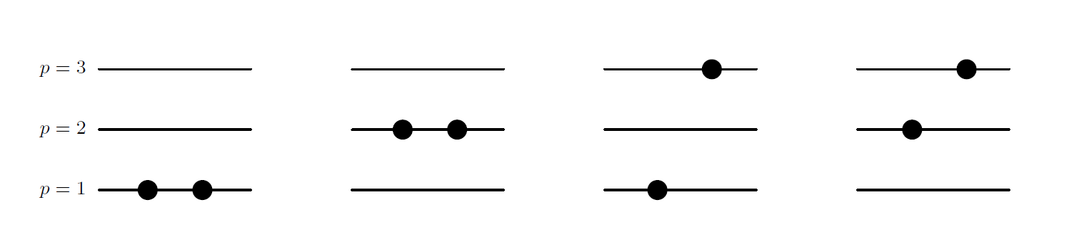
We will now consider a simple three-level problem, depicted in the figure below. This is our first and very simple model of a possible many-nucleon (or just fermion) problem and the shell-model. The single-particle states are labelled by the quantum number \( p \) and can accomodate up to two single particles, viz., every single-particle state is doubly degenerate (you could think of this as one state having spin up and the other spin down). We let the spacing between the doubly degenerate single-particle states be constant, with value \( d \). The first state has energy \( d \). There are only three available single-particle states, \( p=1 \), \( p=2 \) and \( p=3 \), as illustrated in the figure.
a) How many two-particle Slater determinants can we construct in this space? We limit ourselves to a system with only the two lowest single-particle orbits and two particles, \( p=1 \) and \( p=2 \). We assume that we can write the Hamiltonian as $$ \hat{H}=\hat{H}_0+\hat{H}_I, $$ and that the onebody part of the Hamiltonian with single-particle operator \( \hat{h}_0 \) has the property $$ \hat{h}_0\psi_{p\sigma} = p\times d \psi_{p\sigma}, $$ where we have added a spin quantum number \( \sigma \). We assume also that the only two-particle states that can exist are those where two particles are in the same state \( p \), as shown by the two possibilities to the left in the figure. The two-particle matrix elements of \( \hat{H}_I \) have all a constant value, \( -g \).
b) Show then that the Hamiltonian matrix can be written as $$ \left(\begin{array}{cc}2d-g &-g \\ -g &4d-g \end{array}\right), $$
c) Find the eigenvalues and eigenvectors. What is mixing of the state with two particles in \( p=2 \) to the wave function with two-particles in \( p=1 \)? Discuss your results in terms of a linear combination of Slater determinants.
d) Add the possibility that the two particles can be in the state with \( p=3 \) as well and find the Hamiltonian matrix, the eigenvalues and the eigenvectors. We still insist that we only have two-particle states composed of two particles being in the same level \( p \). You can diagonalize numerically your \( 3\times 3 \) matrix.
This simple model catches several birds with a stone. It demonstrates how we can build linear combinations of Slater determinants and interpret these as different admixtures to a given state. It represents also the way we are going to interpret these contributions. The two-particle states above \( p=1 \) will be interpreted as excitations from the ground state configuration, \( p=1 \) here. The reliability of this ansatz for the ground state, with two particles in \( p=1 \), depends on the strength of the interaction \( g \) and the single-particle spacing \( d \). Finally, this model is a simple schematic ansatz for studies of pairing correlations and thereby superfluidity/superconductivity in fermionic systems.
Figure 4: Schematic plot of the possible single-particle levels with double degeneracy. The filled circles indicate occupied particle states. The spacing between each level \( p \) is constant in this picture. We show some possible two-particle states.