12.3. Bayesian methods to deal with outliers

Bayesian approaches to erratic data

We’ll consider four Bayesian approaches to outliers:

1. A conservative model (treat all data points as equally possible outliers).

2. Good-and-bad data model.

3. The Cauchy formulation.

4. Many nuisance parameters.

First, let’s preview our approaches by considering what is problematic about a Gaussian model for the observation errors when we have outliers.

Why are outliers problematic with a Gaussian model?

As noted already, with a Gaussian log likelihood,

\[ \log p(D\mid\boldsymbol{\theta}, I) = \text{constant} - \sum_{i=1}^N \frac{\left[ y_i - y_M(x_i;\boldsymbol{\theta})\right]^2}{2 \sigma_0^2} , \]

in units of \(\sigma_0\) it costs a lot to have an outlier \(y_j\) far from \(y_M(x_j;\boldsymbol{\theta})\) (i.e., to have an outlier with respect to the current model). This distorts the fit of the mean value at \(x_j\), namely \(y_M(x_j;\boldsymbol{\theta})\). Let’s see how that distortion works analytically.

Suppose we first calculate the log likelihood with \(N\) points, none of which are outliers. Then the maximum likelihood parameters \(\boldsymbol{\widehat\theta}\) are such that

\[ \left.\frac{\partial}{\partial\theta_n} \log p(D\mid\boldsymbol{\theta}, I)\right|_{\boldsymbol{\theta} = \boldsymbol{\widehat\theta}} = 0 \quad \text{for each } \theta_n \in \boldsymbol{\theta}. \]

Now hold \(\boldsymbol{\widehat\theta}\) fixed but add a new outlier point \((x_j,y_j)\). What happens to the maximum likelihood condition? Only the new term in the sum will contribute because the derivatives of the other will sum to zero when \(\boldsymbol{\theta} = \boldsymbol{\widehat\theta}\). So now

\[\begin{split}\begin{align} \left.\frac{\partial}{\partial\theta_n} \log p(D\mid\boldsymbol{\theta}, I)\right|_{\boldsymbol{\theta} = \boldsymbol{\widehat\theta}} &= \left.\frac{\partial}{\partial\theta_n} \biggl[-\frac{1}{2}\frac{\bigl(y_j - y_M(x_j;\boldsymbol{\theta})\bigr)^2}{\sigma_0^2} \biggr] \right|_{\boldsymbol{\theta} = \boldsymbol{\widehat\theta}} \\ &= -\left. \frac{y_{j}-y_M(x_j;\boldsymbol{\widehat\theta})}{\sigma_0^2} \frac{\partial y_M(x_j;\boldsymbol{\theta})}{\partial\theta_n} \right|_{\boldsymbol{\theta} = \boldsymbol{\widehat\theta}} , \end{align}\end{split}\]

where only the first factor depends on \(y_j\). Thus this factor will grow without bound:

\[ \frac{y_{j}-y_M(x_j;\boldsymbol{\widehat\theta})}{\sigma_0^2} \overset{y_{j}\rightarrow\infty}{\longrightarrow} \infty , \]

and therefore the parameters in \(\boldsymbol{\widehat\theta}\) are pulled more and more by the single outlier point as the magnitude of the outlier grows. This influence will be the case for any theoretical model, but is intrinsic to the normal distribution for the likelihoo. How to avoid it?

One possibility is to switch to a heavier-tailed distribution that doesn’t have this property of unbounded influence. For example, replace the normal distribution by Student’s t-distribution (here this is any \(i\)):

\[ y_i \sim t_\nu(\mu, \sigma) \quad \Longrightarrow \quad p(y_i | \mu, \sigma^2) \propto \Bigl[ 1 + \frac{(y_i-\mu)^2}{\nu\sigma^2} \Bigr] , \]

with \(\mu = y_M(x_i;\boldsymbol{\theta})\) and \(\sigma = \sigma_0\) here. Then

\[ \log p(y_i | \mu, \sigma^2) = \text{const.} - \frac{\nu+1}{2}\log\Bigl(1 + \frac{(y_i - \mu)^2}{\nu\sigma^2} \Bigr) , \]

and the contribution of \(y_j\) to the minimization of the likelihood is (substituting for \(\mu\) and \(\sigma\))

\[\begin{split}\begin{align} \left.\frac{\partial}{\partial\theta_n} \log p(y_j | y_M(x_j;\boldsymbol{\theta}), \sigma_0^2)\right|_{\boldsymbol{\theta} = \boldsymbol{\widehat\theta}} &= \frac{\nu+1}{2} \frac{1}{1 + (y_j - y_M(x_j;\boldsymbol{\widehat\theta}))^2/\nu\sigma_0^2}\frac{2(y_j - y_M(x_i;\boldsymbol{\widehat\theta}))}{\nu\sigma_0^2} \\ &= \frac{\nu+1}{\nu\sigma_0^2 + (y_j - y_M(x_j;\boldsymbol{\widehat\theta}))^2} (y_j - y_M(x_i;\boldsymbol{\widehat\theta})) . \end{align}\end{split}\]

The t-distribution becomes a Gaussian distribution as \(\nu \rightarrow \infty\), and we see that in that case the derivative will go to infinity like \(y_j - y_M(x_j;\boldsymbol{\widehat\theta})\), as we saw earlier. But for any finite \(\nu\), the \(\bigl(y_j - y_M(x_j;\boldsymbol{\widehat\theta})\bigr)^2\) factor in the denominator with dominate over the \(\nu\sigma_0^2\) factor, and the derivative will vanish as \(y_j \rightarrow \infty\). In other words, the influence on the parameters from the outlier will go away.

In the next section we will see how a heavy-tailed distribution, such as the Student t distribution, can naturally arise in a Bayesian formulation when the uncertainty is itself uncertain.

Approach no. 1: A conservative formulation

Assuming that the specified error bars, \(\sigma_0\), can be viewed as a recommended lower bound, we can construct a more conservative posterior through a marginal likelihood (that is, we introduce \(\sigma\) as a supplementary parameter for what might be the true error, then integrate over it):

\[ p(D_i|\boldsymbol{\theta}, \sigma_0, I) = \int_0^\infty p(D_i|\boldsymbol{\theta},\sigma,I) \, p(\sigma|\sigma_0) \, d\sigma, \]

Note that \(\sigma_0\) doesn’t appear in the first pdf in the integrand and \(\boldsymbol{\theta}\) doesn’t appear in the second pdf. The prior is a variation of Jeffrey’s prior for a scale parameter (which would be \(1/\log(\sigma_1/\sigma_0) \times (1/\sigma)\) for \(\sigma_0 \leq \sigma < \sigma_1\) and zero otherwise),

\[ p(\sigma|\sigma_0,I) = \frac{\sigma_0}{\sigma^2}, \]

for \(\sigma \geq \sigma_0\) and zero otherwise. (This enables us to do the integral up to infinity.) Conservative here means that we treat all data points with suspicion (i.e., we do not single out any points).

The likelihood for a single data point \(D_i\), given by \((x_i,y_i,\sigma_i=\sigma_0)\), is then

(12.2)\[\begin{align} p(D_i | \boldsymbol{\theta}, \sigma_0, I) &= \int_{\sigma_0}^{\infty} \frac{1}{\sqrt{2\pi}\sigma} e^{-\sigma_0^2 R_i^2/2\sigma^2}\, \frac{\sigma_0}{\sigma^2}\, d\sigma \\ &= \frac{\sigma_0}{\sqrt{2\pi}}\int_0^{1/\sigma_0} t \, e^{-t^2 \sigma_0^2 R_i^2/2}\, dt \\ &= \frac{1}{\sigma_0\sqrt{2\pi}} \left[ \frac{1-\exp(-R_i^2/2)}{R_i^2} \right], \end{align}\]

with \(R_i\) the residual as defined above.

Treating the measurement noise as independent, and assigning a uniform prior for the model parameters, we find the log-posterior pdf

\[ \log \left[ p(\boldsymbol{\theta}|D, I)\right] = \text{constant} + \sum_{i=1}^N \log \left[ \frac{1-\exp(-R_i^2/2)}{R_i^2}\right]. \]

We’ll also consider a Cauchy distribution for comparison.

Show code cell source

Hide code cell source

%matplotlib inline

import numpy as np
import matplotlib.pyplot as plt
import seaborn as sns; sns.set(); sns.set_context("talk")

import emcee
import corner
from scipy import optimize

# note that x and y will be used as global arrays
x = np.array([ 0,  3,  9, 14, 15, 19, 20, 21, 30, 35,
             40, 41, 42, 43, 54, 56, 67, 69, 72, 88])
y = np.array([33, 68, 34, 34, 37, 71, 37, 44, 48, 49,
             53, 49, 50, 48, 56, 60, 61, 63, 44, 71])
sig0 = 3.
e = sig0*np.ones_like(y)


def single_gaussian_likelihood(R_i, sigma_0):
   """
   This likelihood is a zero-mean gaussian with standard deviation sigma_0.
   """
   rsq = R_i**2
   return np.exp(-rsq / 2.) / (sigma_0 * np.sqrt(2 * np.pi ))

def single_conservative_likelihood(R_i, sigma_0):
   """
   This likelihood is the result of marginalizing over the standard 
   deviation sigma from sigma0 to infinity with a prior sigma0 / sigma^2.
   """
   rsq = R_i**2
   return (1-np.exp(-rsq / 2.)) / (sigma_0 * np.sqrt(2. * np.pi) * rsq)

def single_cauchy_likelihood(R_i, sigma_0):
   """
   This likelihood is a Cauchy distribution.
   """
   rsq = R_i**2
   return 1 / (sigma_0 * np.pi * np.sqrt(2) * (1. + rsq / 2.))


r = np.linspace(-7, 7)

fig, ax = plt.subplots(1, 1, figsize=(8,6))

ax.plot(r, single_gaussian_likelihood(r,sig0), label="Gaussian", 
       lw=2, ls='--')
ax.plot(r, single_conservative_likelihood(r,sig0), label="Conservative", 
       lw=2, ls='-')
ax.plot(r, single_cauchy_likelihood(r,sig0), label="Cauchy", 
       lw=2, ls='-.')
ax.set(ylabel='Likelihood contribution',xlabel='Residual')
ax.legend(loc='best');

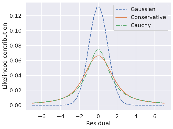
So by marginalizing over the error for each data point, we introduce long tails into the likelihood. The likelihood function is close to a Cauchy distribution in the tails, which is a particular case of a Student \(t\) distribution. (Remember the radioactive lighthouse!)

Now we can sample using this conservative posterior and compare to the others.

If we wanted to get a general Student’s t-distribution, we can do an integration of the variance over an inverse-gamma distribution or, equivalently, integrate over the inverse of the variance with a gamma distribtion. An animation of the integration leading to a t-distribution is created in Student’s t-distribution from Gaussians.

Approach no. 2: Good-and-bad data

In this approach, we are less pessimistic about the data. In particular, we allow for two possibilities:
a) the datum and its error are reliable;
b) the datum is bad and the error should be larger by a (large) factor \(\gamma\).

We implement this with the pdf for \(\sigma\):

\[ p(\sigma | \sigma_0, \beta, \gamma, I) = \beta\, \delta(\sigma - \gamma\sigma_0) + (1-\beta)\, \delta(\sigma - \sigma_0) \;, \]

where \(\beta\) and \(\gamma\) represent the frequency of quirky measurements and their severity. If we use Gaussian pdfs for the two cases, then the likelihood for a datum \(D_i\) after integrating over \(\sigma\) is

\[ p(D_i | \theta, \sigma_0, \beta, \gamma, I) = \frac{1}{\sigma_0 \sqrt{2\pi}} \left\{ \frac{\beta}{\gamma}\, e^{-R_i^2/2\gamma^2} + (1-\beta)\, e^{-R_i^2/2} \right\} \]

We won’t provide code for this approach here but leave it to an exercise (see Sivia, Ch. 8.3.2 for more details). However, we will generalize the idea to the extreme in approach #4 below.

Approach no. 3: The Cauchy formulation

In this approach, we assume \(\sigma \approx \sigma_0\) but allow it to be either narrower or wider:

\[ p(\sigma | \sigma_0, I) = \frac{2\sigma_0}{\sqrt{\pi}\sigma^2} e^{-\sigma_0^2/\sigma^2} \;. \]

Marginalizing \(\sigma\) (using \(\sigma = 1/t\)) gives the Cauchy form likelihood (this is a special case of the Student \(t\) distribution):

\[ p(D_i | \boldsymbol{\theta}, \sigma_0, I) = \frac{1}{\sigma_0 \pi \sqrt{2} [1 + R_i^2(\boldsymbol{\theta})/2]} \;. \]

The log posterior is

\[ L(\boldsymbol{\theta}) = \mbox{constant} - \sum_{i=1}^N \log\left[1 + \frac{R_i^2(\boldsymbol{\theta})}{2}\right] \]

Sampling to compare methods

We’ll use the emcee sampler to generate MCMC samples of our posteriors.

Show code cell source

Hide code cell source

def residuals(theta, x=x, y=y, sigma0=sig0):
    """
    Residuals between data y (a vector at points x) and the theoretical model,
    which here is a straight line with theta[0] = b and theta[1] = m.
    """
    delta_y = y - theta[0] - theta[1] * x
    return delta_y / sigma0

 
def log_posterior_gaussian(theta):
    """
    Returns the logarithm of the posterior, with a standard chi^2 likelihood 
    in terms of the residuals, with Gaussian errors as specified and a
    uniform prior assumed for theta between 0 and 100.
    """
    if (all(theta > 0) and all(theta < 100)):
        return -0.5 * np.sum(residuals(theta)**2)
    else:
        return -np.inf  # recall log(0) = -inf    



def squared_loss(theta, x=x, y=y, sigma0=sig0):
    """Loss function is sum of squared residuals divided by 2, which
        is what we usually call chi^2 / 2. 
    """
    delta_y = y - theta[0] - theta[1] * x
    return np.sum(0.5 * (delta_y / sigma0) ** 2)

# Find the maximum likelihood estimate (MLE) for theta by minimizing the
#  square_loss function using scipy.optimize.fmin. (Minimizing chi^2 gives
#  the same result as maximizing e^{chi^2/2}.)
theta_MLE = optimize.fmin(squared_loss, [0, 0], disp=False)
# Plot the MLE fit versus the data

# Conservative error likelihood
def log_posterior_conservative(theta):
    """
    Log posterior with uniform prior for theta and a Gaussian likelihood
    """
    if (all(theta > 0) and all(theta < 100)):
        r2 = residuals(theta)**2
        return np.sum( np.log((1-np.exp(-r2/2))/r2) )
    else:
        return -np.inf  # recall log(0) = -inf    

# Cauchy likelihood
def log_posterior_cauchy(theta):
    """
    Log posterior with Cauchy likelihood and uniform prior for theta
    """
    if (all(theta > 0) and all(theta < 100)):
        R_sq = residuals(theta)**2
        return - np.sum( np.log(1 + R_sq/2) )
    else:
        return -np.inf  # recall log(0) = -inf    

print('emcee sampling (version: )', emcee.__version__)

ndim = 2 # number of parameters in the model
nwalkers = 10  # number of MCMC walkers
nwarmup = 1000  # "burn-in" period to let chains stabilize
nsteps = 10000  # number of MCMC steps to take

print(f'{nwalkers} walkers:')

# Starting guesses close to the MLE
starting_guesses = np.abs(np.random.normal(1, 1, (nwalkers, 2)))
starting_guesses[:,0] += theta_MLE[0]
starting_guesses[:,1] /= 10
starting_guesses[:,1] += theta_MLE[1]

logps = [log_posterior_gaussian, log_posterior_conservative,
         log_posterior_cauchy]
approaches = ['Std Gaussian', 'Conservative','Cauchy']
mean_68CR = []

for ilogp,logp in enumerate(logps):
    print(f"Log posterior: {approaches[ilogp]}")
    # Sample the posterior distribution
    sampler = emcee.EnsembleSampler(nwalkers, ndim, logp)

    # Warm-up
    if nwarmup > 0:
        print(f'... EMCEE sampler performing {nwarmup} warnup iterations.')
        pos, prob, state = sampler.run_mcmc(starting_guesses, nwarmup)
        sampler.reset()
    else:
        pos = starting_guesses
    
    # Perform iterations, starting at the final position from the warmup.
    print(f'... EMCEE sampler performing {nsteps} samples.')
    %time sampler.run_mcmc(pos, nsteps)
    print("done")

    samples = sampler.flatchain
    lnposts = sampler.lnprobability
    
    # Extract mean and 68% CR
    th0_mcmc, th1_mcmc = map(lambda v: (v[1], v[2]-v[1], v[1]-v[0]),
                             zip(*np.percentile(samples, [16, 50, 84],
                                                axis=0)))
    mean_68CR.append((th0_mcmc,th1_mcmc))
    
    # make a corner plot with the posterior distribution
    fig, ax = plt.subplots(2,2, figsize=(10,10))
    corner.corner(samples,labels=[r"$\theta_0$", r"$\theta_1$"],
                       quantiles=[0.16, 0.5, 0.84],fig=fig,
                       show_titles=True, title_kwargs={"fontsize": 12});
    plt.show()


fig = plt.figure(figsize=(8,6))
ax = fig.add_subplot(1,1,1)
ax.errorbar(x, y, sig0, fmt='o')
xfit = np.linspace(0, 100)
yfit = theta_MLE[0] + theta_MLE[1] * xfit

t = np.linspace(-20, 20)

def huber_loss(t, c=3):
    """
    Returns either a squared lost function or a linear (abolute value) loss
     function, depending on whether the |argument| is < c or >= c.
    """
    return ((abs(t) < c) * 0.5 * t ** 2
            + (abs(t) >= c) * -c * (0.5 * c - abs(t)))

def total_huber_loss(theta, x=x, y=y, sigma0=sig0, c=3):
    return huber_loss((y - theta[0] - theta[1] * x) / sigma0, c).sum()

# minimize the total Huber loss for c=3
theta2 = optimize.fmin(total_huber_loss, [0, 0], disp=False)


print("Summary:             Mean offset  68% CR     Mean slope     68% CR")
for i,approach in enumerate(approaches):
    ((th0,th0pos,th0neg),(th1,th1neg,th1pos)) = mean_68CR[i]
    print(f"{approach:>20s}    {th0:5.2f}   -{th0neg:4.2f},+{th0pos:4.2f}",\
         f"    {th1:5.3f}    -{th1neg:5.3f},+{th1pos:5.3f}")
    ax.plot(xfit, th0 + th1 * xfit, label=approach,  ls='-.')
    
ax.plot(xfit, theta_MLE[0] + theta_MLE[1] * xfit, 
        color='gray',ls='--',label='MLE')
ax.plot(xfit, theta2[0] + theta2[1] * xfit, 
        color='gray',ls='-',label='Huber')
ax.legend(loc='best');

emcee sampling (version: ) 3.1.6
10 walkers:
Log posterior: Std Gaussian
... EMCEE sampler performing 1000 warnup iterations.

... EMCEE sampler performing 10000 samples.

CPU times: user 4.08 s, sys: 1.49 ms, total: 4.08 s
Wall time: 4.08 s
done

Log posterior: Conservative
... EMCEE sampler performing 1000 warnup iterations.

... EMCEE sampler performing 10000 samples.

CPU times: user 4.68 s, sys: 130 μs, total: 4.68 s
Wall time: 4.68 s
done

Log posterior: Cauchy
... EMCEE sampler performing 1000 warnup iterations.

... EMCEE sampler performing 10000 samples.

CPU times: user 4.49 s, sys: 163 μs, total: 4.49 s
Wall time: 4.49 s
done

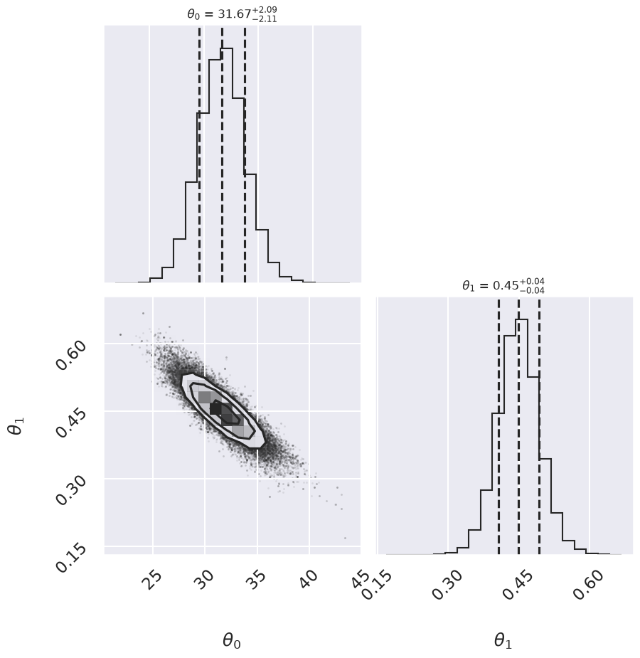
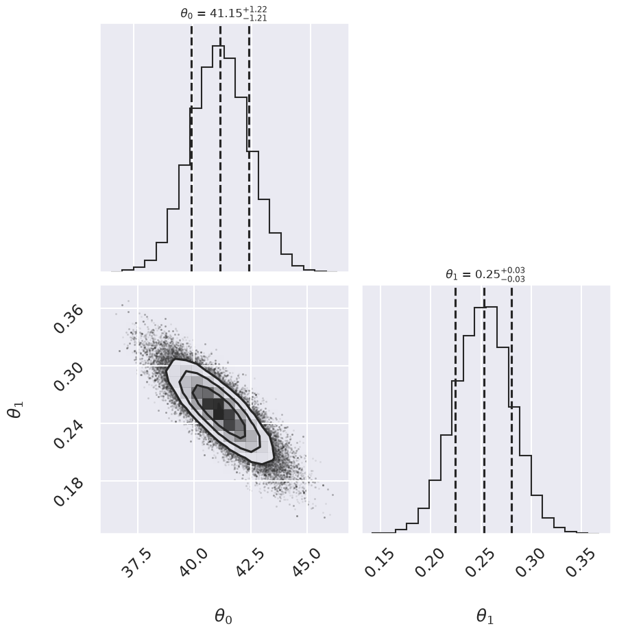
Summary:             Mean offset  68% CR     Mean slope     68% CR
        Std Gaussian    41.16   -1.22,+1.23     0.253    -0.028,+0.028
        Conservative    31.74   -2.28,+2.26     0.448    -0.049,+0.051
              Cauchy    31.54   -2.01,+2.07     0.452    -0.043,+0.042

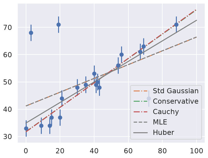
In this plot we see a comparison of five approaches. The standard Gaussian and MLE lines are the same, showing the deleterious effect of the outliers. The Huber loss approach gives a reasonable fit (by eye). The conservative and Cauchy fits are indistinguishable and similar but not identical to the Huber loss fit. Which do you think is better?

Approach no. 4: Many nuisance parameters

The Bayesian approach to accounting for outliers generally involves modifying the model so that the outliers are accounted for. For this data, it is abundantly clear that a simple straight line is not a good fit to our data. So let’s propose a more complicated model that has the flexibility to account for outliers. One option is to choose a mixture between a signal and a background:

\[\begin{split} \begin{array}{ll} p(\{y_i\}~|~\{x_i\}, \{e_i\},~\boldsymbol{\theta},\{g_i\},\sigma_B) = & \frac{g_i}{\sqrt{2\pi e_i^2}}\exp\left[\frac{-\left(\hat{y}(x_i~|~\boldsymbol{\theta}) - y_i\right)^2}{2e_i^2}\right] \\ &+ \frac{1 - g_i}{\sqrt{2\pi \sigma_B^2}}\exp\left[\frac{-\left(\hat{y}(x_i~|~\boldsymbol{\theta}) - y_i\right)^2}{2\sigma_B^2}\right] \end{array} \end{split}\]

What we’ve done is expanded our model with some nuisance parameters: \(\{g_i\}\) is a series of weights which range from 0 to 1 and encode for each point \(i\) the degree to which it fits the model. \(g_i=0\) indicates an outlier, in which case a Gaussian of width \(\sigma_B\) is used in the computation of the likelihood. This \(\sigma_B\) can also be a nuisance parameter, or its value can be set at a sufficiently high number, say 50.

Our model is much more complicated now: it has 22 free parameters rather than 2, but the majority of these can be considered nuisance parameters, which can be marginalized-out in the end, just as we marginalized (integrated) over \(p\) in the Billiard example. Let’s construct a function which implements this likelihood. We’ll use the emcee package to explore the parameter space.

To actually compute this, we’ll start by defining functions describing our prior, our likelihood function, and our posterior:

Now we’ll run the MCMC sampler to explore the parameter space:

Once we have these samples, we can exploit a very nice property of the Markov chains. Because their distribution models the posterior, we can integrate out (i.e. marginalize) over nuisance parameters simply by ignoring them!

We can look at the (marginalized) distribution of slopes and intercepts by examining the first two columns of the sample:

Show code cell source

Hide code cell source

# theta will be an array of length 2 + N, where N is the number of points
# theta[0] is the intercept, theta[1] is the slope,
# and theta[2 + i] is the weight g_i

def log_prior(theta):
    #g_i needs to be between 0 and 1
    if (all(theta[2:] > 0) and all(theta[2:] < 1)):
        return 0
    else:
        return -np.inf  # recall log(0) = -inf

def log_likelihood(theta, x, y, e, sigma_B):
    dy = y - theta[0] - theta[1] * x
    g = np.clip(theta[2:], 0.001, 0.999)  # g<0 or g>1 leads to NaNs in logarithm
    logL1 = np.log(g) - 0.5 * np.log(2 * np.pi * e**2) - 0.5 * (dy / e)**2
    logL2 = np.log(1 - g) - 0.5 * np.log(2 * np.pi * sigma_B**2) \
            - 0.5 * (dy / sigma_B)**2
    return np.sum(np.logaddexp(logL1, logL2))

def log_posterior(theta, x, y, e, sigma_B):
    return log_prior(theta) + log_likelihood(theta, x, y, e, sigma_B)

# Note that this step will take a few minutes to run!

ndim = 2 + len(x)  # number of parameters in the model
nwalkers = 50  # number of MCMC walkers
nburn = 10000  # "burn-in" period to let chains stabilize
nsteps = 15000  # number of MCMC steps to take

# set theta near the maximum likelihood, with 
np.random.seed(0)
starting_guesses = np.zeros((nwalkers, ndim))
starting_guesses[:, :2] = np.random.normal(theta_MLE, 1, (nwalkers, 2))
starting_guesses[:, 2:] = np.random.normal(0.5, 0.1, (nwalkers, ndim - 2))

sampler = emcee.EnsembleSampler(nwalkers, ndim, log_posterior, 
                                args=[x, y, sig0, 50])
sampler.run_mcmc(starting_guesses, nsteps)

samples = sampler.chain[:, nburn:, :].reshape(-1, ndim)


fig, ax = plt.subplots(2,2, figsize=(10,10))
# plot a corner plot with the posterior distribution
# Note that the intercept and the slope correspond to 
#  the first two entries in the parameter array.
fig = corner.corner(samples[:,:2], labels=[r"$\theta_0$", r"$\theta_1$"],
                    quantiles=[0.16, 0.5, 0.84],fig=fig,
                    show_titles=True, title_kwargs={"fontsize": 12})

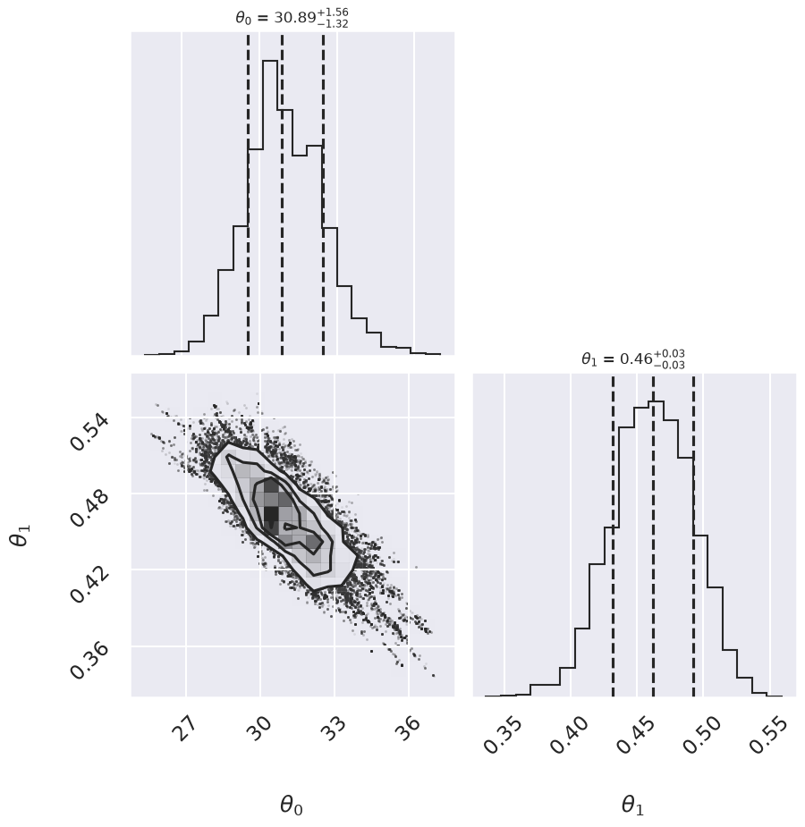
We see a distribution of points near a slope of \(\sim 0.4-0.5\), and an intercept of \(\sim 29-34\). We’ll plot this model over the data below, but first let’s see what other information we can extract from this trace.

One nice feature of analyzing MCMC samples is that the choice of nuisance parameters is completely symmetric: just as we can treat the \(\{g_i\}\) as nuisance parameters, we can also treat the slope and intercept as nuisance parameters! Let’s do this, and check the posterior for \(g_1\) and \(g_2\), the outlier flag for the first two points:

Show code cell source

Hide code cell source

fig, ax = plt.subplots(2,2, figsize=(10,10))
# plot a corner plot with the posterior distribution
# Note that the intercept and the slope correspond to 
#  the first two entries in the parameter array.
fig = corner.corner(samples[:,2:4], labels=[r"$g_1$", r"$g_2$"],
                    quantiles=[0.16, 0.5, 0.84],fig=fig,
                    show_titles=True, title_kwargs={"fontsize": 12})

print("g1 mean: {0:.2f}".format(samples[:, 2].mean()))
print("g2 mean: {0:.2f}".format(samples[:, 3].mean()))

g1 mean: 0.65
g2 mean: 0.39

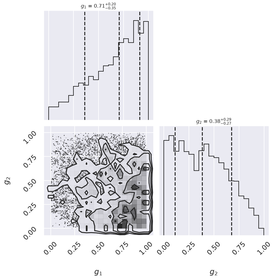
There is not an extremely strong constraint on either of these, but we do see that \((g_1, g_2) = (1, 0)\) is slightly favored: the means of \(g_1\) and \(g_2\) are greater than and less than 0.5, respectively. If we choose a cutoff at \(g=0.5\), our algorithm has identified \(g_2\) as an outlier.

Let’s make use of all this information, and plot the marginalized best model over the original data. As a bonus, we’ll draw red circles to indicate which points the model detects as outliers:

Show code cell source

Hide code cell source

theta3 = np.mean(samples[:, :2], 0)
g = np.mean(samples[:, 2:], 0)
outliers = (g < 0.5)

fig = plt.figure(figsize=(8,6))
ax = fig.add_subplot(1,1,1)
ax.errorbar(x, y, sig0, fmt='o')

ax.plot(xfit, theta3[0] + theta3[1] * xfit, color='black')
ax.scatter(x[outliers], y[outliers], 
            marker='o', s=150, edgecolors='r', linewidths=4, c='k',
            label='Bayesian #4')

ax.plot(xfit, theta_MLE[0] + theta_MLE[1] * xfit, 
        color='gray',ls='--',label='MLE')
ax.plot(xfit, theta2[0] + theta2[1] * xfit, 
        color='gray',ls='-',label='Huber')
ax.legend(loc='best');

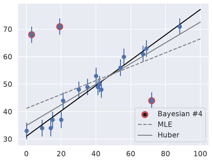
The result, shown by the dark line, matches our intuition! Furthermore, the points automatically identified as outliers are the ones we would identify by hand. For comparison, the gray lines show the two previous approaches: the simple maximum likelihood and the frequentist approach based on Huber loss.

Discussion

Here we’ve dived into linear regression in the presence of outliers. A typical Gaussian maximum likelihood approach fails to account for the outliers, but we were able to correct this in the frequentist paradigm by modifying the loss function, and in the Bayesian paradigm by adopting a mixture model with a large number of nuisance parameters.

Both approaches have their advantages and disadvantages: the frequentist approach here is relatively straightforward and computationally efficient, but is based on the use of a loss function which is not particularly well-motivated. The Bayesian approach is well-founded and produces very nice results, but it is much more intensive in both coding time and computational time. It also requires a specification of a prior that must be motivated. The advantage is that this prior choice can be tested and compared to alternatives. While you will often see this choice described in the literature (mostly older literature now) as “subjective”, in fact it is a more objective approach because of the ability to evaluate it!