11.1. Indifferences and translation groups#
Discrete permutation invariance#
Consider a six-sided dice
How do we assign \(p_i \equiv p(X_i|I)\), \(i \in \{1, 2, 3, 4, 5, 6\}\)?
We do know \(\sum_i p(X_i|I) = 1\)
Invariance under labeling \(\Rightarrow p(X_i|I)=1/6\)
provided that the prior information \(I\) says nothing that breaks the permutation symmetry (e.g., we might know that the dice are not fair).
Location invariance#
Indifference to a constant shift \(x_0\) for a location parameter \(x\) implies that
in the allowed range.
Location invariance implies that
Provided that the prior information \(I\) says nothing that breaks the symmetry.
The pdf will be zero outside the allowed range (specified by \(I\)).
Scale invariance#
Indifference to a re-scaling \(\lambda\) of a scale parameter \(x\) implies that
in the allowed range.
Invariance under re-scaling implies that
Provided that the prior information \(I\) says nothing that breaks the symmetry.
The pdf will be zero outside the allowed range (specified by \(I\)).
This prior is often called a Jeffrey’s prior; it represents a complete ignorance of a scale parameter within an allowed range.
It is equivalent to a uniform pdf for the logarithm: \(p(\log(x)|I) = \mathrm{constant}\)
as can be verified with a change of variable \(y=\log(x)\), see lecture notes on error propagation.
Checkpoint question
Can you provide alternative evidence for the scale invariance result?
Answer
scale invariance \(\longrightarrow\) \(p(x|I) \propto 1/x\)
First check that it works: \(p(x|I) = \lambda p(\lambda x|I)\) \(\Lra\) \(\frac{c}{x} = \frac{\lambda c}{\lambda x} = \frac{c}{x}\). Check!
Now a more general proof: assume \(p(x|I) \propto x^{\alpha}\). Then \(x^\alpha = \lambda (\lambda x)^{\alpha} = \lambda^{1+\alpha} x^\alpha\) \(\Lra\) \(\alpha = -1\). Check!
Still more general: set \(\lambda = 1 + \epsilon\) with \(\epsilon \ll 1\), and solve to \(\mathcal{O}(\epsilon)\): \(p(x) = (1+\epsilon)(p(x)+\epsilon\frac{dp}{dx})\) \(\Lra\) \(p(x) + x \frac{dp}{dx} = 0\)
so \(p(x) \propto 1/x\).
Example: Straight-line model#
Consider the theoretical model
Would you consider the intercept \(\theta_0\) a location or a scale parameter, or something else?
Would you consider the slope \(\theta_1\) a location or a scale parameter, or something else?
Consider also the statistical model for the observed data \(y_i = y_\mathrm{th}(x_i) + \epsilon_i\), where we assume independent, Gaussian noise \(\epsilon_i \sim \mathcal{N}(0, \sigma^2)\).
Would you consider the standard deviation \(\sigma\) a location or a scale parameter, or something else?
Symmetry invariance#
In fact, by symmetry indifference we could as well have written the linear model as \(x_\mathrm{th}(y) = \theta_1' y + \theta_0'\)
We would then equate the probability elements for the two models
The transformation gives \((\theta_0', \theta_1') = (-\theta_1^{-1}\theta_0, \theta_1^{-1})\).
This change of variables implies that
where the (absolute value of the) determinant of the Jacobian is
In summary we find that \(\theta_1^3 p(\theta_0, \theta_1 | I) = p(-\theta_1^{-1}\theta_0, \theta_1^{-1}|I).\)
This functional equation is satisfied by
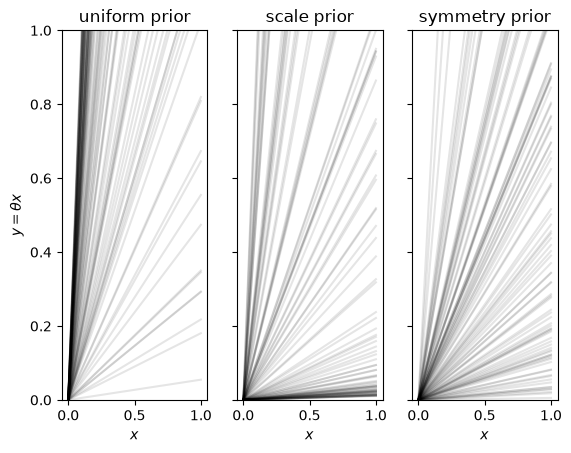
Fig. 11.1 100 samples of straight lines with fixed intercept equal to 0 and slopes sampled from three different prior pdfs. Note in particular the prior preference for large slopes that results from using a uniform pdf.#
Straight-line example with MCMC sampling#
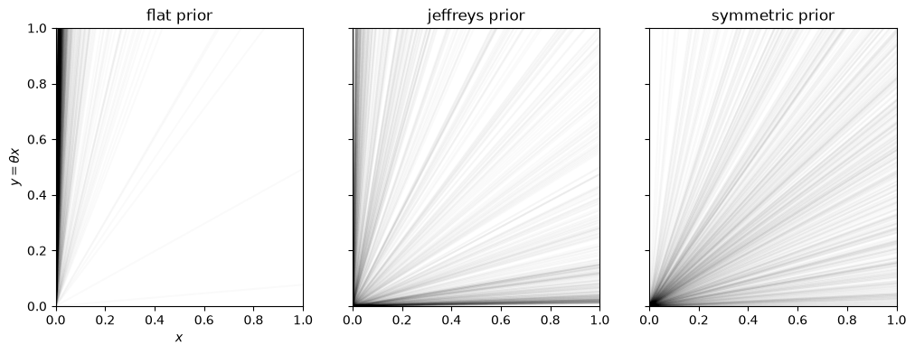
We will define three different priors for the straight line model. Using always a flat prior U(-100,100) for the intercept, and a non-zero pdf range -100 <= slope <= 100. For the scale-invariant (Jeffreys) prior we must also exclude a small region around zero slope (here 0.01 < |slope|) since 1/|slope| is not normalizable otherwise.
Let us create 1000 samples from each prior pdf and plot the resulting sample of straight lines. Since the intercept is uniformly distributed in all three prior alternatives, we will just consider straight lines with intercept 0 since it makes it easier to compare the distribution of slopes.
MCMC sampling of log_flat_prior using emcee with 10 walkers
Mean acceptance fraction: 0.827 (in total 100000 steps)
MCMC sampling of log_jeffreys_prior using emcee with 10 walkers
Mean acceptance fraction: 0.586 (in total 100000 steps)
MCMC sampling of log_symmetric_prior using emcee with 10 walkers
Mean acceptance fraction: 0.776 (in total 100000 steps)