21.3. Demo: MCMC Diagnostics

This notebook demonstrates some of the basic MCMC diagnostic tools.

import numpy as np
from scipy.stats import norm, uniform

import matplotlib.pyplot as plt

import pandas as pd
import warnings
warnings.filterwarnings('ignore')

MCMC diagnostics: assessing convergence

From previous notebooks we know that MCMC sampling is a powerful tool for Bayesian inference. However, MCMC samples represent the posterior only once the chain has converged to its stationary distribution. Convergence is guaranteed in the limit of infinitely many steps, but a finite chain can still be far from stationary, or explore the posterior so slowly that its samples are strongly correlated. Since we cannot simply inspect the posterior, we rely on a set of numerical diagnostics that detect when something is wrong. None of them can prove convergence, but together they flag many problematic scenarios.

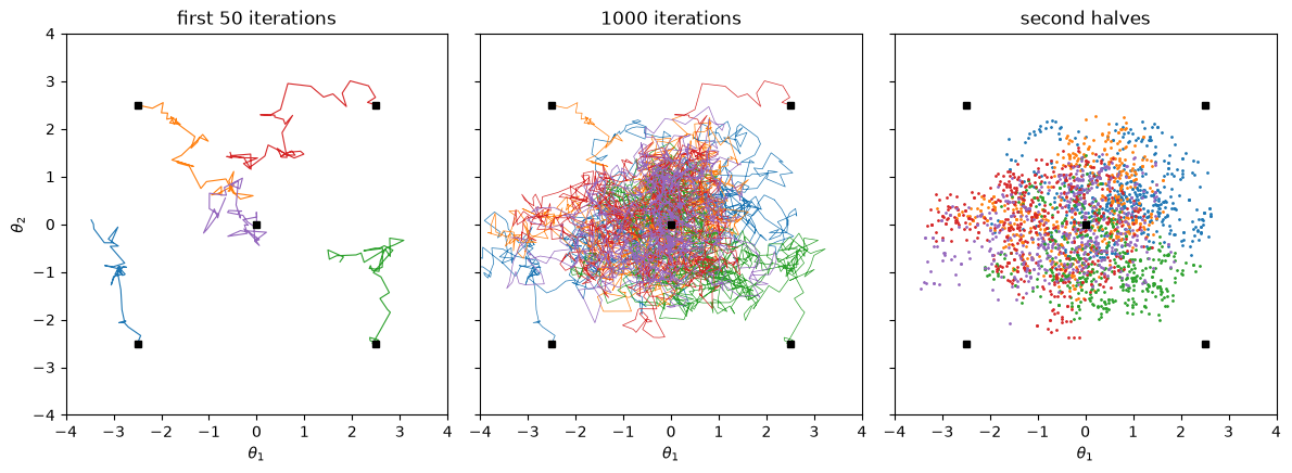
The figure generated with the following code shows five Metropolis chains sampling a bivariate normal distribution, started from overdispersed points. After 50 iterations the chains are still far from the target and from each other (left panel); after 1000 iterations they have mixed (middle panel), and the second halves of the chains look like samples from the target (right panel).

# Our own version of BDA3 Fig. 11.1: five Metropolis chains sampling a
# bivariate unit normal, started from overdispersed points.
def metropolis(log_p, theta0, nsteps, proposal_width, rng):
    """Random-walk Metropolis with a Gaussian proposal; returns the chain."""
    theta = np.array(theta0, dtype=float)
    logp = log_p(theta)
    chain = np.empty((nsteps + 1, len(theta)))
    chain[0] = theta
    for i in range(1, nsteps + 1):
        proposal = theta + proposal_width * rng.standard_normal(len(theta))
        logp_prop = log_p(proposal)
        if np.log(rng.uniform()) < logp_prop - logp:
            theta, logp = proposal, logp_prop
        chain[i] = theta
    return chain

log_target = lambda th: -0.5 * th @ th   # bivariate unit normal
starts = [(-2.5, -2.5), (-2.5, 2.5), (2.5, -2.5), (2.5, 2.5), (0., 0.)]
rng = np.random.default_rng(1)
chains = [metropolis(log_target, th0, 1000, 0.2, rng) for th0 in starts]

fig, axs = plt.subplots(1, 3, figsize=(12, 4.5), sharex=True, sharey=True)
for ch in chains:
    axs[0].plot(ch[:51, 0], ch[:51, 1], '-', lw=0.8)
    axs[1].plot(ch[:, 0], ch[:, 1], '-', lw=0.5)
    axs[2].plot(ch[501:, 0], ch[501:, 1], '.', ms=2)
for ax, title in zip(axs, ['first 50 iterations', '1000 iterations', 'second halves']):
    ax.plot(*zip(*starts), 'ks', ms=4)   # starting points
    ax.set_title(title)
    ax.set_xlabel(r'$\theta_1$')
    ax.set_xlim(-4, 4); ax.set_ylim(-4, 4); ax.set_aspect('equal')
axs[0].set_ylabel(r'$\theta_2$')
fig.tight_layout()

Fitting a straight line - revisited

Let us revisit the problem of inferring the parameters of a straight line. See also 📥 Problem: fitting a straight line and 📥 Problem: fitting a straight line II

The Data

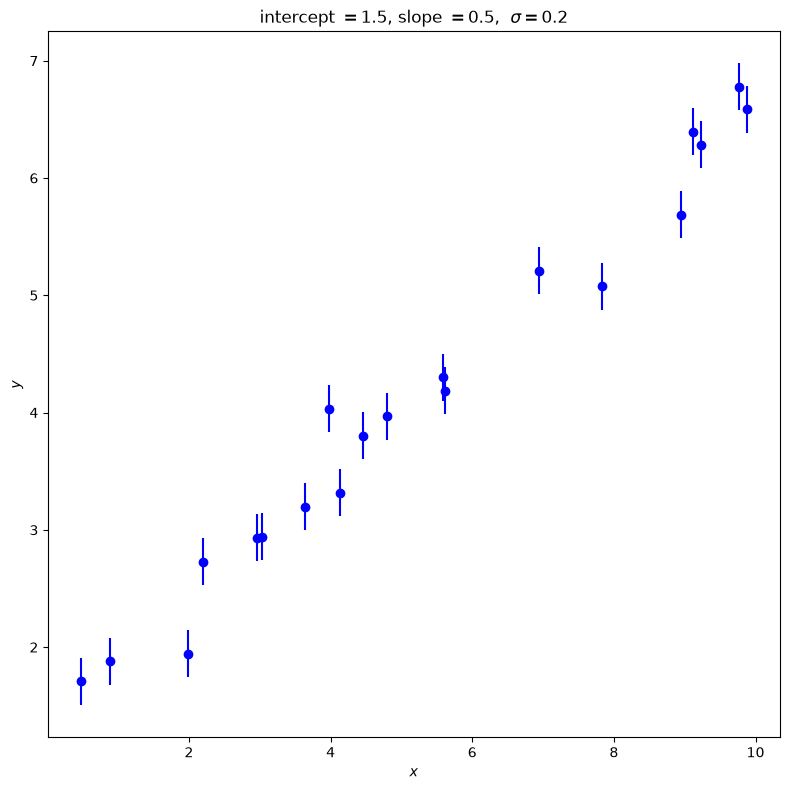
We start by creating some data that we will fit with a straight line. The data is generated with a variance \(\sigma^2\) on the \(y\) values and no error on \(x\).

def make_data(intercept, slope, N_pts=20, dy=.2, rseed=None):
    """Given a straight line defined by intercept and slope:
          y = slope * x + intercept
       generate N_pts points randomly spaced points from x=0 to x=x_max
       with Gaussian (i.e., normal) error with mean zero and standard
       deviation dy.
       
       Unless rseed is specified as an integer, new random data will be 
       generated each time.
       
       Return the x and y arrays and an array of standard deviations.
    """
    rand = np.random.RandomState(rseed) 
    
    x_max = 10.
    x = x_max * rand.rand(N_pts)  # choose the x values randomly in [0,10]
    y = intercept + slope * x  # This is the y value without noise
    y += dy * rand.randn(N_pts)    # Add in Gaussian noise
    return x, y, dy * np.ones_like(x)  # return coordinates and error bars

# Fix the random seed so that the data and the MCMC runs are reproducible.
# (emcee draws from numpy's global random state unless given its own.)
seed = 2026
np.random.seed(seed)

# Specify the true parameters and make sample data
intercept = 1.5   # true intercept (called b elsewhere)
slope = 0.5       # true slope (called m elsewhere)
theta_true = [intercept, slope]  # put parameters in a true theta vector
x, y, dy = make_data(*theta_true, rseed=seed)

# Make a plot of the data
fig, ax = plt.subplots(figsize=(8,8))
ax.errorbar(x, y, dy, fmt='o', color='blue')
ax.set_xlabel(r'$x$')
ax.set_ylabel(r'$y$')
plot_title = rf'intercept $= {intercept:.1f}$, slope $= {slope:.1f}$, ' \
              + rf' $\sigma = {dy[0]:.1f}$'
ax.set_title(plot_title)
fig.tight_layout()

The Model

Next we need to specify a theoretical model. We’re fitting a straight line to data, so we’ll need a slope and an intercept; i.e.

\[ y_{\textrm{th}}(x) = mx + b \]

where our parameter vector will be

\[ \theta = [b, m] \]

But this is only half the picture: what we mean by a “model” in a Bayesian sense is not only this expected value \(y_{\textrm{th}}(x;\theta)\), but a probability distribution for our data. That is, we need an expression to compute the likelihood \(p(D\mid\theta, I)\) for our data as a function of the parameters \(\theta\) (\(I\) stands for all other information). Here \(D\) is the set of all \((x,y)\) pairs that we know about (or measure).

[Note: At this stage we are (implicitly) assuming that our theoretical model is perfect. But it is not! We’ll come back eventually to talk about adding a theory error \(\delta y_{\textrm{th}}\).]

We are given data with simple error bars, which imply that the probability for any single data point (labeled by \(i\)) is a normal distribution with mean given by the true value. That is,

\[ y_i \sim \mathcal{N}(y_{\textrm{th}}(x_i;\theta), \varepsilon_i^2) \]

or, in other words,

\[ p(y_i\mid x_i,\theta, I) = \frac{1}{\sqrt{2\pi\varepsilon_i^2}} \exp\left(\frac{-\left[y_i - y_{\textrm{th}}(x_i;\theta)\right]^2}{2\varepsilon_i^2}\right) \]

where \(\varepsilon_i\) are the (known) measurement errors indicated by the error bars.

Assuming all the points are independent, we can find the full likelihood by multiplying the individual likelihoods together:

\[ p(D\mid\theta, I) = \prod_{i=1}^N p(y_i\mid x_i,\theta, I) \]

For convenience (and also for numerical accuracy) this is often expressed in terms of the log-likelihood:

\[ \log p(D\mid\theta, I) = -\frac{1}{2}\sum_{i=1}^N\left(\log(2\pi\varepsilon_i^2) + \frac{\left[y_i - y_M(x_i;\theta)\right]^2}{\varepsilon_i^2}\right) \]

# Log likelihood
def log_likelihood(theta, x, y, dy):
    """Return the log likelihood given the vector of parameters theta and
        numpy arrays for x, y, and dy (which is the standard deviation).
    """
    y_model = theta[0] + theta[1] * x
    return -0.5 * np.sum(np.log(2 * np.pi * dy ** 2) + 
                         (y - y_model) ** 2 / dy ** 2)

# Let's use the (log) symmetric prior, which is the scale-invariant one.
# Uniform prior for the offset
def log_prior(theta):
    """Prior p(m) proportional to (1 + m^2)^{-3/2}"""
    if np.abs(theta[0]) < 1000:
        return -1.5 * np.log(1 + theta[1]**2)
    else:
        return -np.inf  # log(0)
    
def log_posterior(theta, x, y, dy):
    """Return the log posterior by evaluating the log prior and log
        likelihood.
       Probably should first check if the log prior is -np.inf before 
        evaluating the log likelihood
    """
    return log_prior(theta) + log_likelihood(theta, x, y, dy)

We will use the emcee sampler, but in its Metropolis-Hastings mode. In particular, we invoke the sampler with moves.GaussianMove(cov), which implements a Metropolis step using a Gaussian proposal with mean zero and covariance cov. The covariance cov could be a scalar, as it is here, or a vector or a matrix. See the relevant emcee manual page for further details and more general moves. The stepsize parameter is at our disposal to explore the consequences on convergence of it being too large or too small.

One consequence of this choice deserves emphasis. With emcee’s default stretch move, a walker’s proposal is constructed from the positions of the other walkers, so the walkers in the ensemble are not independent chains. A Gaussian Metropolis proposal, in contrast, depends only on the walker’s own current position. In this notebook each walker is therefore an independent Markov chain, and we will exploit this below when we treat the walkers as separate chains for convergence diagnostics. Do not assume this for an ensemble sampler in general.

Alternatively, you can use your own sampler here if you created one.

import emcee
import corner
print('emcee sampling (version: )', emcee.__version__)

ndim = 2  # number of parameters in the model
nwalkers = 10
nwarmup = 1000
nsteps = 5000

# MH-Sampler setup
stepsize = .005
cov = stepsize * np.eye(ndim)
p0 = np.random.rand(nwalkers,ndim)

# initialize the sampler
sampler = emcee.EnsembleSampler(nwalkers, ndim, log_posterior, args=[x, y, dy],
                               moves=emcee.moves.GaussianMove(cov))

emcee sampling (version: ) 3.1.6

To get the chains below we use sampler.get_chain(), which returns an array with the shape (# steps, # walkers, # dimensions). So 10 walkers taking 5000 steps each for a two-dimensional posterior (that is, \(\boldsymbol{\theta}\) has two components) gives the shape (5000, 10, 2). We can combine the results from all the walkers with sampler.get_chain(flat=True), which flattens the first two axes so that the array has the shape (# steps \(\times\) # walkers, # dimensions). Note that the flattened samples are ordered step by step (all walkers at step 0, then all walkers at step 1, and so on). The flattened array is therefore fine for histograms and corner plots, but for trace plots we use the unflattened array and draw one line per walker. The log-posterior values are obtained in the same way with sampler.get_log_prob().

# Sample the posterior distribution

# Warm-up
if nwarmup > 0:
    print(f'Performing {nwarmup} warmup iterations.')
    pos, prob, state = sampler.run_mcmc(p0, nwarmup)
    sampler.reset()
else:
    pos = p0
    
# Perform iterations, starting at the final position from the warmup.
print(f'MH sampler performing {nsteps} samples.')
%time sampler.run_mcmc(pos, nsteps)
print("done")

print(f"Mean acceptance fraction: {np.mean(sampler.acceptance_fraction):.3f}")

# get_chain() has shape (nsteps, nwalkers, ndim); flat=True merges the first two axes
samples = sampler.get_chain(flat=True)
samples_unflattened = sampler.get_chain()
lnposts = sampler.get_log_prob(flat=True)
lnposts_unflattened = sampler.get_log_prob()

    
# make a corner plot with the posterior distribution
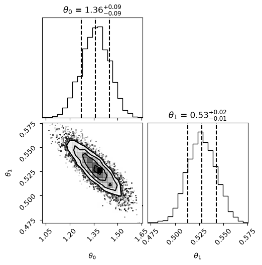
fig = corner.corner(samples, quantiles=[0.16, 0.5, 0.84], labels=[r"$\theta_0$", r"$\theta_1$"],
                       show_titles=True, title_kwargs={"fontsize": 12})

Performing 1000 warmup iterations.

MH sampler performing 5000 samples.

CPU times: user 1.62 s, sys: 2.11 ms, total: 1.62 s
Wall time: 1.62 s
done
Mean acceptance fraction: 0.113

print(samples.shape)
print(samples_unflattened.shape)
print(lnposts.shape)
print(lnposts_unflattened.shape)

(50000, 2)
(5000, 10, 2)
(50000,)
(5000, 10)

fix, ax = plt.subplots(3,2,figsize=(12,5*ndim))
for irow in range(ndim):
    # one line per walker
    ax[irow,0].plot(samples_unflattened[:,:,irow], alpha=0.5)
    ax[irow,0].set_ylabel(r'$\theta_{0}$'.format(irow))
    ax[irow,1].hist(samples[:,irow],orientation='horizontal',bins=30)
    
ax[2,0].plot(lnposts_unflattened, alpha=0.5)
ax[2,1].hist(lnposts,orientation='horizontal',bins=30)
ax[2,0].set_ylabel(r'$\log(p)$')
ax[2,0].set_xlabel('step')

ax[0,1].set_title('Histogram')
ax[0,0].set_title('Trace Plot')

plt.tight_layout()

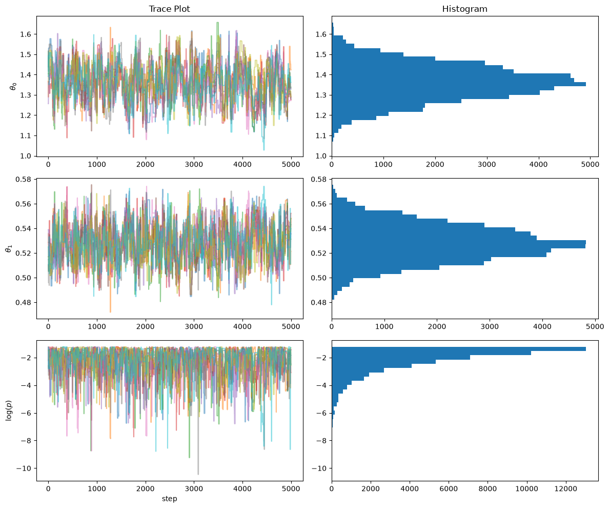
How do we know this chain has converged to the posterior?

Credit to BDA3 by Gelman et al. and lecture notes by Rob Hicks

Standard Error of the Mean

This investigates the question how does the mean of \(\theta\) deviate in our chain, and is capturing the simulation error of the mean rather than underlying uncertainty of our parameter \(\theta\):

\[ SE({\bar{\theta}}) = \frac{\text{Posterior Standard Deviation}}{\sqrt{N}} \]

where \(N\) is the chain length (the number of iterations in your chain).

For our problem this is:

for irow in range(ndim):
    print(f"Standard Error of the Mean for theta_{irow}: {samples[:,irow].std()/np.sqrt(samples.shape[0]):.1e}")

Standard Error of the Mean for theta_0: 3.9e-04
Standard Error of the Mean for theta_1: 6.5e-05

This is saying that very little of our posterior variation in \(\theta\) is due to sampling error (that is good). We can visualize this by examining the moving average of a chain as we move through the iterations. Since each walker is an independent chain here (because of the Metropolis move, see above), we study a single walker (the flattened array interleaves the walkers and is not a time series):

# with the Gaussian Metropolis move each walker is an independent chain; shape (nsteps, ndim)
chain0 = samples_unflattened[:, 0, :]

fix, ax = plt.subplots(2,1,figsize=(12,10))
# pandas makes this easy:
df_chain = pd.DataFrame(chain0,columns=['theta0','theta1'])
df_chain['ma_theta0'] = df_chain.theta0.rolling(window=100,center=False).mean()
df_chain['ma_theta1'] = df_chain.theta1.rolling(window=100,center=False).mean()

ax[0].plot(np.arange(chain0.shape[0]),chain0[:,0],label=r'$\theta_0$')
ax[0].plot(np.arange(chain0.shape[0]),df_chain['ma_theta0'],label=r'Moving average')
ax[0].set_ylabel(r'$\theta_0$')

ax[1].plot(np.arange(chain0.shape[0]),chain0[:,1],label=r'trace')
ax[1].plot(np.arange(chain0.shape[0]),df_chain['ma_theta1'],label=r'Moving average')
ax[1].set_ylabel(r'$\theta_1$')
ax[1].set_xlabel('step')

plt.legend();

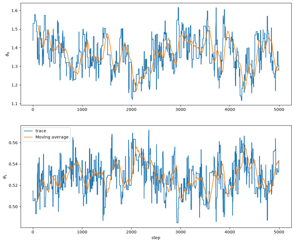
This is a good sign that our chain is stable, since both the individual samples of \(\theta\) in our chain and the mean of the samples dance around a stable value of \(\theta\). The calculation above makes this more concrete. There are time series versions of this calculation that accounts for the fact that the chain is not iid.

Autocorrelation Plots

def autocorrelation(chain, max_lag=100):
    dimension = len(chain)
    acors = np.empty(max_lag+1)
    if max_lag > len(chain)/5:
        warnings.warn('max_lag is more than one fifth the chain length')
    # Create a copy of the chain with average zero
    chain1d = chain - np.average(chain)
    for lag in range(max_lag+1):
        unshifted = None
        shifted = chain1d[lag:]
        if 0 == lag:
            unshifted = chain1d
        else:
            unshifted = chain1d[:-lag]
        normalization = np.sqrt(np.dot(unshifted, unshifted))
        normalization *= np.sqrt(np.dot(shifted, shifted))
        acors[lag] = np.dot(unshifted, shifted) / normalization
    return acors

fig, ax = plt.subplots(1,2,sharey=True,figsize=(12,5))
for icol in range(ndim):
    # autocorrelation along a single walker's chain
    max_lag = 300
    acors = autocorrelation(chain0[:,icol],max_lag=max_lag)
    ax[icol].plot(acors, label='our estimate')
    # emcee's built-in estimate of the same function (FFT based)
    acors_emcee = emcee.autocorr.function_1d(chain0[:,icol])
    ax[icol].plot(acors_emcee[:max_lag+1], '--', label='emcee.autocorr.function_1d')
    ax[icol].set_xlabel('lag')
ax[0].set(ylabel='autocorrelation', ylim=(-.5, 1.));
ax[0].legend();

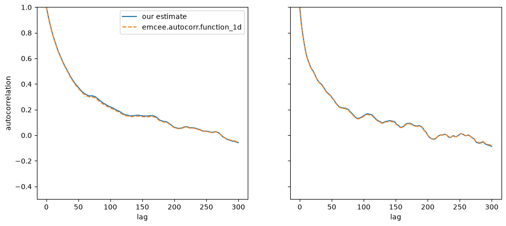
The two estimates agree (they differ only in the normalization of the lagged sums). A more compact summary is the integrated autocorrelation time \(\tau\), roughly the number of steps between effectively independent samples. emcee estimates it from all walkers with sampler.get_autocorr_time(). Note that the estimate is only considered reliable when the chain is longer than about \(50\tau\); for a shorter chain emcee raises an error unless quiet=True, in which case it warns and returns the estimate anyway.

tau = sampler.get_autocorr_time(quiet=True)
for irow in range(ndim):
    print(f"Integrated autocorrelation time for theta_{irow}: {tau[irow]:.0f} steps")
print(f"Effective number of independent samples: ~{nsteps*nwalkers/np.max(tau):.0f} (out of {nsteps*nwalkers})")

Integrated autocorrelation time for theta_0: 50 steps
Integrated autocorrelation time for theta_1: 42 steps
Effective number of independent samples: ~993 (out of 50000)

Standard error of the mean, revisited

The standard error of the mean computed above assumed \(N\) independent samples. With correlated samples the effective number is only \(N/\tau\), so the error should be \(\sigma\sqrt{\tau/N}\). We can check this directly: the walkers are independent chains with our Metropolis move (again, not for the default stretch move), so the scatter of the walker means measures the actual simulation error of a single-chain mean, and dividing by \(\sqrt{n_\mathrm{walkers}}\) gives the error of the combined mean.

N = samples.shape[0]
walker_means = samples_unflattened.mean(axis=0)   # shape (nwalkers, ndim)
for irow in range(ndim):
    sigma = samples[:,irow].std()
    se_naive = sigma / np.sqrt(N)
    se_tau = sigma * np.sqrt(tau[irow] / N)
    se_empirical = walker_means[:,irow].std(ddof=1) / np.sqrt(nwalkers)
    print(f"theta_{irow}: SE assuming independent samples = {se_naive:.1e},"
          f"  corrected with tau = {se_tau:.1e},"
          f"  from the spread of walker means = {se_empirical:.1e}")

theta_0: SE assuming independent samples = 3.9e-04,  corrected with tau = 2.8e-03,  from the spread of walker means = 2.5e-03
theta_1: SE assuming independent samples = 6.5e-05,  corrected with tau = 4.2e-04,  from the spread of walker means = 3.9e-04

Acceptance Rate for the MH Algorithm

Recall that we want the acceptance rate to be in the range .2 to .4. For our problem this paper suggests an acceptance rate of .234 for random walk MH.

Since the number of new members in the chain represent the number of acceptances, count changes in chain values and divide by total chain length to calculate acceptance rate:

print(f"Acceptance Rate is: {np.mean(sampler.acceptance_fraction):.3f}")

Acceptance Rate is: 0.113

The acceptance rate is helpful in describing convergence because it indicates a good level of “mixing” over the parameter space. The acceptance rate can be tuned via the proposal width after which we re-run our MH MCMC sampler.

Note: modern software (like pymc and emcee) can auto-tune the proposal distribution to achieve a desired acceptance rate.

Gelman Rubin Diagnostic

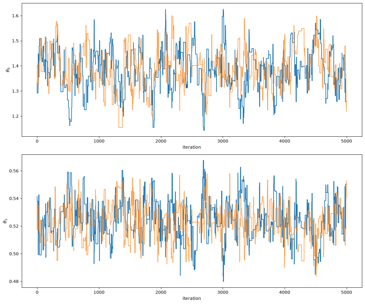
If our MH MCMC Chain reaches a stationary distribution, and we repeat the exercise multiple times, then we can examine if the posterior for each chain converges to the same place in the distribution of the parameter space.

Steps:

1. Run multiple chains starting at different points (multiple walkers). Discard the warm-up for each.

2. Split each chain in two, with \(N\) iterations in each half chain. Call \(M\) the total number of chains now (twice the original number).

3. Calculate the within and between chain variance. This tests both mixing (if well-mixed, the separate parts of different chains should mix) and stationarity (two halves of each chain should be sampling the same distribution).

• Label the scalar parameter or expectation value being tested as \(\psi\) and label the simulated results as \(\psi_{ij}\), where \(i\) runs from 1 to \(N\) within each chain and \(j\) labels the chain from 1 to \(M\). Then we define:

\[ \overline\psi_{\cdot j} \equiv \frac{1}{N} \sum_{i=1}^{N} \psi_{ij} \quad \mbox{and} \quad \overline\psi_{\cdot \cdot} \equiv \frac{1}{M} \sum_{j=1}^{M} \overline\psi_{\cdot j} \]

where \(\overline\psi_{\cdot j}\) is the mean within chain \(j\) and \(\overline\psi_{\cdot \cdot}\) is the average (mean) of these means across the \(M\) chains.

• Within chain variance:

\[ W = \frac{1}{M}\sum_{j=1}^M s_j^2 \quad \mbox{where} \quad s_j^2 = \frac{1}{N-1}\sum_{i=1}^{N}(\psi_{ij} - \overline\psi_{\cdot j})^2 \;, \]

with \(s_j^2\) is the variance of each chain. So \(W\) is the mean of the in-chain variances. It is expected that \(W\) will underestimate the variance of \(\psi\) (which we’ll denote \({\mbox{var}}(\psi)\) because an individual sequence (i.e., chain) with \(N < \infty\) will not have run forever, so it will not have ranged over the full target distribution, so it will have less variability.

• Between chain variance:

\[ B = \frac{N}{M-1} \sum_{j=1}^M (\overline\psi_{\cdot j} - \overline\psi_{\cdot \cdot})^2 \;. \]

There is an \(N\) in the numerator of \(B\) because it is from the variance of the within-sequence means \(\overline\psi_{\cdot j}\), each of which is an average of \(N\) values \(\psi_{ij}\).

4. Calculate the estimated variance of \(\psi\) as the weighted sum of within and between chain variance.

\[ \hat{\mbox{var}}(\psi)^{+} = \left ( 1 - \frac{1}{N}\right ) W + \frac{1}{N}B \;. \]

This quantity is expected to overestimate \({\mbox{var}}(\psi)\) but is unbiased under stationarity.

5. Calculate the potential scale reduction factor, \(\hat{R}\), which is the factor by which the scale that characterizes the distribution for \(\psi\) at the current stage might be reduced if we increased each chain size \(N\) toward infinity:

\[ \hat{R} = \sqrt{\frac{\hat{\mbox{var}}(\psi)}{W}} \]

Based on our expectations, this should be greater than 1 because the numerator overestimates \({\mbox{var}}(\psi)\) and denominator underestimates it. But if it is close to 1, then it should mean that both chains are mixing around the stationary distribution.
Gelman and Rubin show that when \(\hat{R}\) is greater than 1.1 or 1.2, we need longer runs.

Let’s run 2 chains:

no_of_chains=2
chains=[]

for ichain in range(no_of_chains):
    sampler.reset()
    p0 = np.random.rand(nwalkers,ndim)
    # Warm-up
    if nwarmup > 0:
        print(f'Chain {ichain} performing {nwarmup} warmup iterations.')
        pos, prob, state = sampler.run_mcmc(p0, nwarmup)
        sampler.reset()
    else:
        pos = p0
    
    # Perform iterations, starting at the final position from the warmup.
    print(f'MH sampler {ichain} performing {nsteps} samples.')
    sampler.run_mcmc(pos, nsteps)
    print("done")
    print(f"Mean acceptance fraction: {np.mean(sampler.acceptance_fraction):.3f}")

    # With the Gaussian Metropolis move each walker is an independent chain
    # (not true for emcee's default stretch move!). We keep one walker (index 0)
    # as the chain from this run; shape (nsteps, ndim)
    chains.append(sampler.get_chain()[:, 0, :])

Chain 0 performing 1000 warmup iterations.

MH sampler 0 performing 5000 samples.

done
Mean acceptance fraction: 0.117
Chain 1 performing 1000 warmup iterations.

MH sampler 1 performing 5000 samples.

done
Mean acceptance fraction: 0.111

chain1 = chains[0]
chain2 = chains[1]
num_iter = chain1.shape[0]

fig, ax = plt.subplots(2, 1, figsize=(12,10))
for icol in range(ndim):
    ax[icol].plot(np.arange(num_iter), chain1[:,icol])
    ax[icol].plot(np.arange(num_iter), chain2[:,icol], alpha=.7)
    ax[icol].set_ylabel(fr'$\theta_{icol}$')
    ax[icol].set_xlabel('iteration')
    
fig.tight_layout()

# rewrite of Gelman-Rubin estimation
# we only want one of the variables
Nchain = int(nsteps / 2)  # maximum size of each half chain
Mchain = 4   # total number of chains
param = 0    # which parameter to use


def Gelman_Rubin_diagnostic_calc(chains, Nchain, Mchain=4, param=0):
    psi_chains = np.zeros((Mchain, Nchain))
    for icol in range(0, Mchain, 2):
        i = int(icol/2)
        psi_chains[icol,:] = np.array( chains[i] )[:Nchain, param]
        psi_chains[icol+1,:] = np.array( chains[i] )[Nchain:2*Nchain, param]
    
    psi_mean = np.array([chain.mean() for chain in psi_chains])
    psi_mean_all = psi_mean.sum() / Mchain

    var_chain = np.zeros(Mchain)
    for i in range(Mchain):
        var_chain[i] = 1./(Nchain - 1) * \
                           ((psi_chains[i] - psi_mean[i])**2).sum()

    W = var_chain.sum() / Mchain

    B = Nchain / (Mchain - 1) * \
          np.array([(mean - psi_mean_all)**2 for mean in psi_mean]).sum()
    
    var_theta = (1. - 1./Nchain) * W + 1./Nchain * B
    Rhat = np.sqrt(var_theta/W)
    print(fr"Nchain = {Nchain:4d}  Rhat = {Rhat:.3f}")
    
print(f"Gelman-Rubin Diagnostic for different chain lengths: ")
for Nchain in [50, 100, 200, 500, 1000, 2000]:
    Gelman_Rubin_diagnostic_calc(chains, Nchain, param=0)

Gelman-Rubin Diagnostic for different chain lengths: 
Nchain =   50  Rhat = 1.166
Nchain =  100  Rhat = 1.071
Nchain =  200  Rhat = 1.013
Nchain =  500  Rhat = 1.065
Nchain = 1000  Rhat = 1.056
Nchain = 2000  Rhat = 1.003

To repeat: Gelman and Rubin show that when \(\hat{R}\) is greater than 1.1 or 1.2, we need longer runs.

Univariate Approaches

The diagnostics we have discussed are all univariate (they work perfectly when there is only one parameter to estimate).

So most people examine univariate diagnostics for each variable, examine autocorrelation plots, acceptance rates and try to argue chain convergence based on that.