21.1. Workflow for MCMC sampling

MCMC sampling is an enabling technology for modern Bayesian inference. It allows us to collect samples from complex target probability distributions that may be high-dimensional, out of reach for analytical treatment, and computationally costly to evaluate. Here we consider a possible workflow to make MCMC sampling efficient, to diagnose and address possible failure modes, and to make the sampling results interpretable:

Four-phase MCMC workflow

1. Preparatory phase

2. Warmup phase

3. Collection phase

4. Analysis phase

In this section we give a general overview of the four phases. Explicit examples, best practices, and more detailed considerations follow when we discuss specific sampling algorithms in Advanced sampling algorithms and their implementations in State-of-the-art MCMC implementations. The diagnostics referred to here are introduced in Diagnostics for MCMC sampling and demonstrated in Demo: MCMC Diagnostics. For an opinionated practitioner’s account of MCMC in the physical sciences, see Hogg and Foreman-Mackey [HFM18].

The four phases are shown on the left in Fig. 21.1: (1) prepare for sampling by considering all available information about the target distribution; (2) warm up by tuning the sampler and letting the chains equilibrate; (3) collect as many samples as the computational budget allows; (4) analyze the results and provide Monte Carlo estimators for the quantities of interest. Although the phases are traversed in order, there are feedback loops within each phase, and the diagnostic checkpoints can send us back to an earlier phase to start over. The samples collected during warmup are discarded and must not be mixed with those from the collection phase.

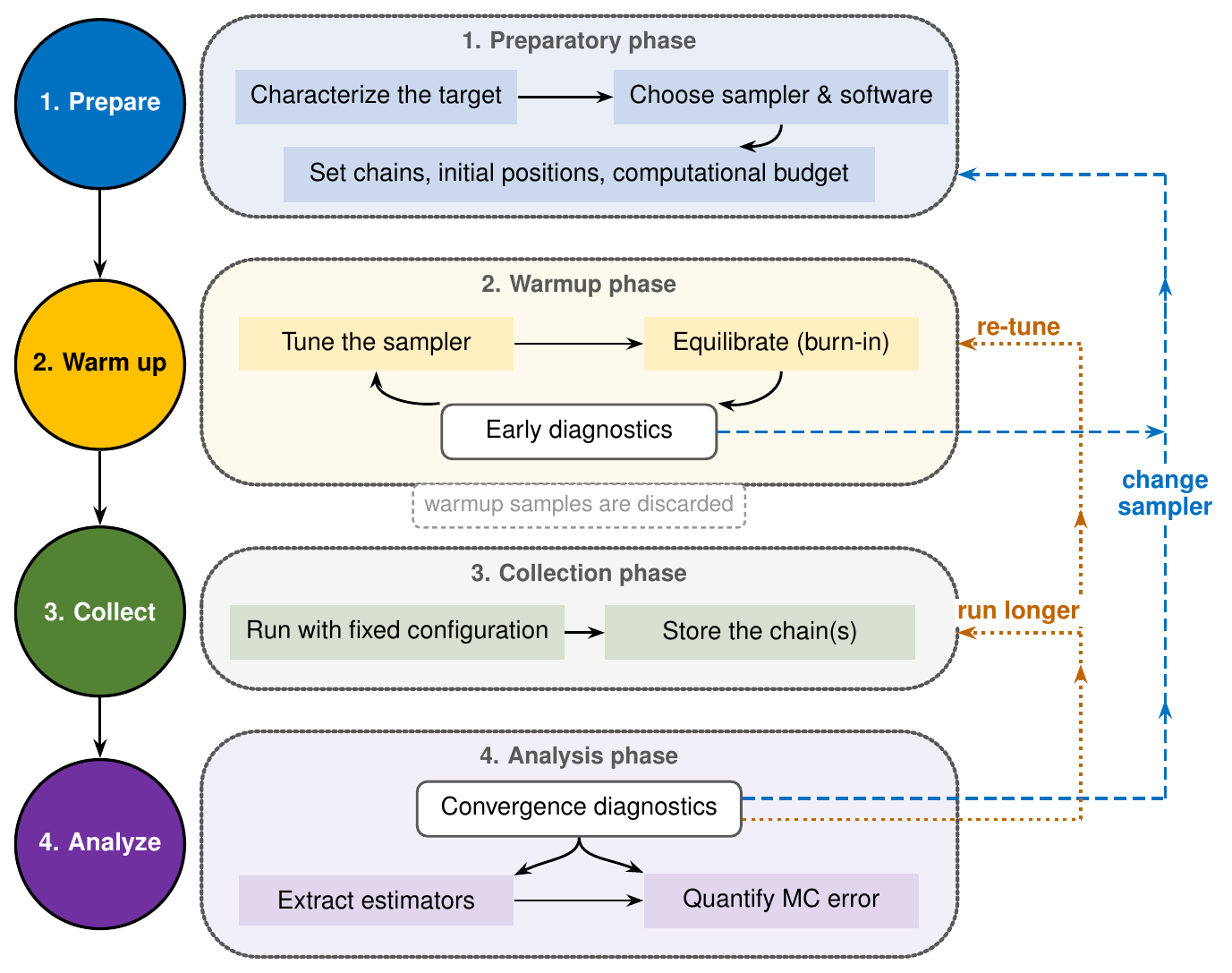
Fig. 21.1 The MCMC workflow. Coloured boxes are actions that belong to one phase, while white outlined boxes are diagnostic checkpoints, from which the dashed feedback paths depart. The short-dashed path returns to the warmup phase (re-tune or run longer), the long-dashed path to the preparatory phase (change sampler).

In the following subsections we expand upon each phase.

Phase 1: Preparatory Phase

In the preparatory phase we characterize the target distribution: its dimension, the cost of a single evaluation, and whether gradients are available. Any prior knowledge of its shape (the regions of high probability mass, strong correlations between parameters, possible multimodality) feeds into the choice of sampling algorithm, the number of chains, and the distribution of initial positions. Since the cost is usually dominated by the likelihood evaluation, the total computational budget sets a firm limit on the number of samples, and the algorithm should be chosen so that this budget buys as many effectively independent samples as possible. Note also that MCMC is a tool for sampling, not for optimization: if the goal is only to locate the mode of a distribution, an optimizer is the better choice [HFM18].

Two practical steps belong here as well. First, verify the implementation of the target before sampling: evaluate the log-probability at a few points, check that it returns \(-\infty\) outside the support (and never NaN) and, when gradients are used, compare them with finite differences. Second, decide what will be recorded during the run. The convergence diagnostics of the later phases are computed from the parameter traces, but only if these are stored per chain and in step order; the log-probability of each sample comes for free and is worth keeping as well, both as an informal diagnostic and for later use.

We take an end-user perspective here: rather than engineering our own Markov transitions we rely on existing, well-tested sampling software, and the choice among these is discussed in State-of-the-art MCMC implementations.

Not every sampling algorithm is of the Markov chain type. Nested sampling (Nested sampling) instead evolves a population of live points that is successively compressed towards regions of higher likelihood; its primary output is the evidence, with weighted posterior samples as a by-product. There is no burn-in, or autocorrelation time in that scheme, so the workflow described here applies to it only in its preparatory and analysis phases, and it has its own convergence criteria.

Phase 2: Warmup phase

The warmup phase consists of two steps, tuning and equilibration, connected through a feedback loop with early diagnostics. In the tuning step we adapt the parameters of the sampling algorithm to the target distribution, as represented by the warmup samples. Which parameters these are depends on the algorithm: for the Metropolis–Hastings algorithm (Derivation of the Metropolis-Hastings algorithm) it is the step length and the functional form of the proposal distribution; for Hamiltonian Monte Carlo (Hamiltonian Monte Carlo) it is the mass matrix, the leapfrog step size, and the number of steps (which, with the step size, sets the integration time). Tuning is critical for performance. Tuning can also mean transforming the parameters: a linear transformation that removes strong correlations, or sampling \(\log\sigma\) instead of a scale parameter \(\sigma\), often helps any sampler more than adjusting its internal settings. Modern sampling software typically performs the adaptation of internal settings automatically during a designated warmup period, but the user still has to judge whether it succeeded. The early diagnostics used for this purpose are acceptance rates, trace plots, and preliminary estimates of the autocorrelation time.

The equilibration step, also known as burn-in, moves the chains from their initial positions, which may lie in an unrepresentative region of parameter space, into the region where the probability mass is concentrated. Starting several chains from dispersed positions makes this step more informative: trace plots and the Gelman–Rubin statistic \(\hat{R}\) (Diagnostics for MCMC sampling) show whether the chains have forgotten where they started and have found the same region. If they have not, a longer warmup is needed; if they have, but the sampler moves too slowly, one returns to tuning; and if tuning cannot fix it, one returns to the preparatory phase and reconsiders the algorithm.

All warmup samples must be discarded. During tuning the transition kernel keeps changing, so the chain is not yet a Markov chain with a fixed stationary distribution, and its samples do not follow the target. The samples collected during equilibration do come from the final kernel, but from its transient regime rather than from its limiting distribution, so they would bias the Monte Carlo estimators. Neither kind may be mixed with the samples of the collection phase.

Phase 3: Collection phase

The collection phase is a long run with fixed sampler configuration, in which we collect as many samples as the computational budget allows. The chain positions are stored per chain and in step order, since this is what the convergence diagnostics of the final phase require; flattened arrays, with all chains pooled, are then used for constructing the Monte Carlo estimators. It is worth also storing the log-probability of every position. It comes for free from the sampler and serves as an additional diagnostic: a chain stuck in a low-probability region, or a \(\log p\) that keeps drifting upward, shows up there before it does in the parameters. It is also needed for identifying the MAP sample and for the evidence-related methods later in the book. Some samplers report further per-step quantities, such as divergent transitions in Hamiltonian Monte Carlo, that are genuinely diagnostic and cannot be reconstructed from the traces; these should be stored as well.

How long should the run be? Since a chain can appear converged while it has not yet discovered a part of the parameter space, the only real safeguard is to run longer than seems necessary. Geyer, in his introduction to the Handbook of Markov Chain Monte Carlo [Gey11], argues for one long run rather than many short ones:

Worse, addiction to many short runs can keep one from running the sampler long enough to detect pseudo-convergence or other problems, such as bugs in the code. People who have used MCMC in complicated problems can tell stories about samplers that appeared to be converging until after weeks of running they discovered a new part of the state space and the distribution changed radically. If those people had thought it necessary to make hundreds of runs, none of them could have been several weeks long.

Geyer makes another recommendation, “only a bit facetious”, for those who write scientific papers based on MCMC sampling:

[O]ne should start a run when the paper is submitted and keep running until referee’s reports arrive. This cannot delay the paper, and may detect pseudo-convergence.

Note that this advice concerns the length of each chain; it does not contradict the use of a handful of chains started from dispersed positions, which is what makes the between-chain diagnostics of the next phase possible.

Phase 4: Analysis phase

The analysis phase begins with the convergence diagnostics of Diagnostics for MCMC sampling, now applied to the full collection run. Between-chain comparisons and \(\hat{R}\) test whether chains started from dispersed positions agree; trace plots and the log-probability trace reveal chains that are stuck or still drifting; and the autocorrelation time \(\tau\), which is only estimated reliably from long chains, tells us how many effectively independent samples we have, \(N_\mathrm{eff} \approx N/\tau\). A long run also increases the chance of exposing problematic behaviour such as multimodality. Passing these checks is a prerequisite for everything that follows; failing them sends us back to the warmup phase (longer run, re-tuning) or, if the sampler is fundamentally unsuited, to the preparatory phase.

Once the samples are trusted, Monte Carlo estimators are formed from the pooled samples of all chains: posterior means and medians, credible intervals from quantiles, and marginal distributions of any subset of parameters, which are obtained simply by ignoring the other coordinates. A corner plot is nothing but the set of one- and two-dimensional marginals. Predictive distributions follow by pushing each sample through the model. The MAP estimate can be read off from the stored log-probabilities, although with finite samples it is only approximate and often less useful than the posterior summaries.

Three plots to make every time you run MCMC

Following Hogg and Foreman-Mackey [HFM18], three figures should accompany every MCMC analysis.

1. Trace plots of all chains expose the equilibration time, problems with the model or the sampler, and give a qualitative impression of convergence.

2. Corner plots show all one- and two-dimensional marginal distributions; they are remarkable for locating expected and unexpected parameter relationships, and often suggest reparametrizations that simplify the problem.

3. Posterior predictive plots compare predictions with a few dozen random samples to the observed data; they give a qualitative sense of how well the model fits and can also expose problems with sampling or convergence.

Every estimator should be reported with its Monte Carlo error, which for a mean is \(\sigma/\sqrt{N_\mathrm{eff}}\) rather than \(\sigma/\sqrt{N}\). Interval endpoints and other tail quantities are more demanding for two reasons: their sampling variance is intrinsically larger than that of a mean, since few samples fall in the tails, and the autocorrelation time of a tail indicator is typically longer than that of the parameter itself, so the relevant \(N_\mathrm{eff}\) is smaller [VGS+21]. A posterior mean is well determined by a few hundred effective samples; the endpoints of a 95% credible interval require thousands. Thinning the chain is not needed for these estimators, since correlated samples carry less information per sample but discarding them never adds information; it is justified only to save storage or to make plots legible.

Finally, the analysis phase hands over to model checking. Whether the posterior itself is reasonable, as judged by posterior predictive checks, sensitivity to the prior, and comparison with alternative models, is the subject of the Bayesian workflow in Bayesian research workflow and is answered with the same set of samples.