\[\newcommand\pos{\boldsymbol{x}} \newcommand\mom{\boldsymbol{p}} \newcommand\mass{\mathcal{M}}\]

21.2. Diagnostics for MCMC sampling

We’ve seen that using MCMC leads to a Markov chain: a set of configurations of the parameters we are sampling. This chain enables inference because they are samples of the posterior of interest. MCMC sampling is notoriously difficult to validate. In this section we discuss the common convergence tests that enter the warmup and analysis phases of the workflow in Workflow for MCMC sampling. Keep in mind that none of them can prove convergence; they can only detect certain kinds of failure. Passing all tests is therefore necessary, but not sufficient.

Convergence tests for MCMC sampling

MCMC sampling can go wrong in (at least) three ways:

1. No convergence—The limiting distribution is not reached.

2. Pseudoconvergence—The chain seems stationary, but the limiting distribution is not actually reached.

3. Highly correlated samples—Not really wrong, but inefficient.

There is no unique solution to such problems, but they are typically addressed in three ways:

1. Design the simulation runs for monitoring of convergence. In particular, run multiple sequences of the Markov chains with starting points dispersed over the sampling space. This is difficult in high dimensions.

2. Monitor the convergence of individual sampling dimensions, as well as predicted quantities of interest, by comparing variations within and between the different sequences (chains). Here you are looking for stationarity (the running means are stable) and mixing (different sequences are sampling the same distribution). The Gelman-Rubin test (see below) is devised for this purpose. Fig. 21.2 illustrates the two failure modes (cf. Figure 11.3 in BDA3 [GCS+13]): on the left two chains that each look stationary but stay in separate regions of \(\theta_0\) (no mixing), and on the right two chains that mix well but drift together, so that neither samples a stationary distribution (the \(\theta_0\) distribution keeps changing with MC steps).

Show code cell source

Hide code cell source

import numpy as np
import matplotlib.pyplot as plt

rng = np.random.default_rng(3)
nsteps = 400
t = np.arange(nsteps)

def ar1(n, mean, sigma, phi, rng):
    """Stationary, autocorrelated noise around a mean (AR(1) process)."""
    x = np.empty(n); x[0] = mean
    for i in range(1, n):
        x[i] = mean + phi * (x[i-1] - mean) + sigma * np.sqrt(1 - phi**2) * rng.standard_normal()
    return x

fig_mix, axs = plt.subplots(1, 2, figsize=(10, 3.6), sharey=True)

# left: stationary but not mixing -- two chains in separate regions
axs[0].plot(t, ar1(nsteps, +1.5, 0.4, 0.9, rng), lw=0.8)
axs[0].plot(t, ar1(nsteps, -1.5, 0.4, 0.9, rng), lw=0.8)
axs[0].set_title('stationary, but not mixing')

# right: mixing but not stationary -- both chains drift together
drift = 2.0 * np.sin(2 * np.pi * t / (2.5 * nsteps))
axs[1].plot(t, drift + ar1(nsteps, 0, 0.5, 0.8, rng), lw=0.8)
axs[1].plot(t, drift + ar1(nsteps, 0, 0.5, 0.8, rng), lw=0.8)
axs[1].set_title('mixing, but not stationary')

for ax in axs:
    ax.set_xlabel('MC step')
axs[0].set_ylabel(r'$\theta_0$')
fig_mix.tight_layout()

from myst_nb import glue
glue("stationarity_mixing_fig", fig_mix, display=False)
plt.close(fig_mix)

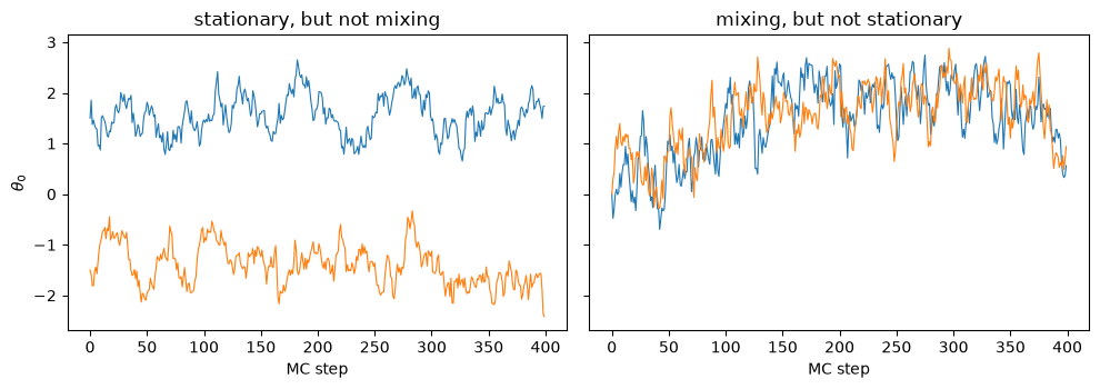
Fig. 21.2 Two ways in which MCMC chains can fail. Left: two chains that are each stationary but sample different regions of parameter space and never mix. Right: two chains that mix but are not stationary, since both drift with the number of MC steps. Only chains that are both stationary and mixing sample the target distribution.

3. Monitor the autocorrelation of the samples (see below), which determines how many effectively independent samples a chain of given length contains. Strong autocorrelation implies that the algorithm must be tuned, or that an altogether different sampling algorithm should be used. A first indicator is the acceptance rate of the sampler: for a random-walk Metropolis sampler an acceptance rate close to one means that the steps are too short (successive samples are almost identical), while a rate close to zero means that almost every proposal is rejected (the chain stands still). The optimal value depends on the algorithm: for random-walk Metropolis proposals values in the range 0.2–0.5 are typically desired in high dimensions; for Hamiltonian Monte Carlo the target is much higher, around 0.65–0.8, since its proposals are informed by the gradient; for the affine-invariant ensemble sampler its authors again recommend 0.2–0.5.

The diagnostics that will be discussed below are all univariate. They work perfectly when there is only one parameter to estimate. In fact, most convergence tests are performed with univariate diagnostics applied to each sampling dimension one by one.

Variance of the mean

Consider the sampling variance of a parameter mean value. If the \(N\) samples were independent draws from the posterior it would be

(21.1)\[ \var{\bar\para} = \frac{\var{\para}}{N}, \]

where \(N\) is the length of the chain. This quantity is capturing the simulation error of the mean rather than the underlying uncertainty of the parameter \(\para\). MCMC samples are not independent, however, and we will see below how the formula must be corrected. We can visualize this by examining the moving average of our parameter trace. The trace is the sequence as a function of iteration number.

Autocorrelation

A challenge when doing MCMC sampling is that the collected samples can be correlated. This can be tested by computing the autocorrelation function and extracting the correlation time for a chain of samples.

Say that \(X\) is an array of \(N\) samples numbered by the index \(t\). Then \(X_{+h}\) is a shifted version of \(X\) with elements \(X_{t+h}\). The integer \(h\) is called the lag. Since we have a finite number of samples, the array \(X_{+h}\) will be \(h\) elements shorter than \(X\).

Furthermore, \(\bar{X}\) is the average value of \(X\).

We can then define the autocorrelation function \(\rho(h)\) from the list of samples.

(21.2)\[ \rho(h) = \frac{\sum_{t=0}^{N-h-1} \left[ (X_t - \bar{X}) (X_{t+h} - \bar{X})\right]} {\sqrt{ \sum_{t=0}^{N-h-1} (X_t - \bar{X})^2 } \sqrt{ \sum_{t=0}^{N-h-1} (X_{t+h} - \bar{X})^2 }} \]

The summation is carried out over the subset of samples that overlap. The autocorrelation is the overlap (scalar product) of the chain of samples (the trace) with a copy of itself shifted by the lag, as a function of the lag. If the lag is short so that nearby samples are close to each other (and have not moved very far) the product of these two vectors is large. If samples are independent, you will have both positive and negative numbers in the overlap that cancel each other.

The typical example of a highly correlated chain is a random walk with a too short proposal step length.

It is often observed that \(\rho(h)\) is roughly exponential so that we can define an autocorrelation time \(\tau_\mathrm{a}\) according to \(\rho(h) \sim \exp(-h/\tau_\mathrm{a})\).

The quantity that enters the error estimates below is instead the integrated autocorrelation time

\[ \tau = 1 + 2 \lim_{N \to \infty} \sum_{h=1}^N \rho(h). \]

For a purely exponential \(\rho(h)\) the two are related by \(\tau \approx 2\tau_\mathrm{a}\) (for \(\tau_\mathrm{a} \gg 1\)), so one should be careful about which one is quoted.

With autocorrelated samples, the sampling variance (21.1) becomes

(21.3)\[ \var{\bar\para} = \tau \frac{\var{\para}}{N}, \]

with \(\tau \gg 1\) for highly correlated samples. This motivates us to define the effective sample size (ESS), or effective number of samples, as

\[ N_\mathrm{eff} = N / \tau. \]

To keep \(N_\mathrm{eff}\) high, we must collect many samples and keep the autocorrelation time small.

In practice \(\tau\) must be estimated from the finite chain, and the naive sum of \(\rho(h)\) over all lags does not work: the estimated \(\rho(h)\) at large lag is pure noise that does not decay, so the sum keeps wandering. The standard remedy, due to Sokal, is to truncate the sum at a window \(M\) chosen self-consistently such that \(M \gtrsim 5\tau\). This is what emcee.autocorr.integrated_time (and thus sampler.get_autocorr_time()) implements, averaging the autocorrelation functions of all walkers before integrating. The estimate is only trustworthy when the chain is much longer than the autocorrelation time, \(N \gtrsim 50\tau\) as a rule of thumb; emcee raises an error otherwise. Finally, \(\tau\) is a property of the quantity whose time series is analyzed, not of the chain alone: the autocorrelation time of a tail indicator \(\mathbb{1}[\para > q]\) is typically longer than that of \(\para\) itself, so tail quantities have a smaller \(N_\mathrm{eff}\) than the per-parameter value suggests [VGS+21].

The Gelman-Rubin test

The Gelman-Rubin diagnostic was constructed to test for stationarity and mixing of different Markov chain sequences [GR92].

Algorithm 21.1 (The Gelman-Rubin diagnostic)

1. Collect \(M>1\) sequences (chains) of length \(2N\).

2. Discard the first \(N\) draws of each sequence, leaving the last \(N\) iterations in the chain.

3. Calculate the within and between chain variance.

   • Within chain variance:

     \[ W = \frac{1}{M}\sum_{j=1}^M s_j^2 \]

     where \(s_j^2\) is the variance of each chain (after throwing out the first \(N\) draws).

   • Between chain variance:

     \[ B = \frac{N}{M-1} \sum_{j=1}^M (\bar{\para}_j - \bar{\bar{\para}})^2 \]

   where \(\bar{\para}_j\) is the mean of chain \(j\) and \(\bar{\bar{\para}}\) is the mean of the \(M\) chain means.

4. Calculate the estimated variance of \(\theta\) as the weighted sum of between and within chain variance.

\[ \widehat{\var{\para}} = \left ( 1 - \frac{1}{N}\right ) W + \frac{1}{N}B \]

5. Calculate the potential scale reduction factor.

\[ \hat{R} = \sqrt{\frac{\widehat{\var{\para}}}{W}} \]

We want the \(\hat{R}\) number to be close to 1 since this would indicate that the between chain variance is small. And a small between chain variance means that the chains are mixing around the same stationary distribution. Gelman and Rubin [GR92] showed that stationarity has certainly not been achieved when \(\hat{R}\) is greater than 1.1 or 1.2. Current practice is stricter and uses the split \(\hat{R}\): each chain is cut into two halves that are treated as separate sequences (so \(M\) chains give \(2M\) sequences), which also detects a chain that is still drifting, and convergence is only accepted for \(\hat{R} < 1.01\) [VGS+21].

Two remarks are in order. First, the test is only meaningful for independent chains started from dispersed positions. The walkers of an ensemble sampler with the default stretch move are not independent (each proposal is constructed from the positions of the other walkers), so \(\hat{R}\) across walkers of a single ensemble is not a valid diagnostic; one has to compare independent ensembles. With a Metropolis move, as in Demo: MCMC Diagnostics, each walker is an independent chain and the test can be applied across walkers. Second, like all the diagnostics discussed here \(\hat{R}\) can give a false pass: chains that have all found the same mode of a multimodal posterior, but none of the others, will happily agree with each other.