12.1. Setup: linear regression with data outliers

We will use as our canonical example a set of data that mostly lies close to a straight line, and is expected to lie on a straight line, but has several points that are far away. (This example and subsequent discussion was adapted from the blog post Frequentism and Bayesianism II: When Results Differ.)

Sample dataset

Consider the following plotted dataset, relating the observed variables \(x\) and \(y\), with errors on \(y\). (You will have the opportunity to explore different datasets and errors in 📥 Demo: Illustrating approaches to outliers.)

Show code cell source

Hide code cell source

%matplotlib inline

import numpy as np
import matplotlib.pyplot as plt
import seaborn as sns; sns.set(); sns.set_context("talk")

import emcee
import corner

# note that x and y will be used as global arrays
x = np.array([ 0,  3,  9, 14, 15, 19, 20, 21, 30, 35,
              40, 41, 42, 43, 54, 56, 67, 69, 72, 88])
y = np.array([33, 68, 34, 34, 37, 71, 37, 44, 48, 49,
              53, 49, 50, 48, 56, 60, 61, 63, 44, 71])
sig0 = 3.
e = sig0*np.ones_like(y)

fig = plt.figure(figsize=(8,6))
ax = fig.add_subplot(1,1,1)
ax.errorbar(x, y, e, fmt='o');

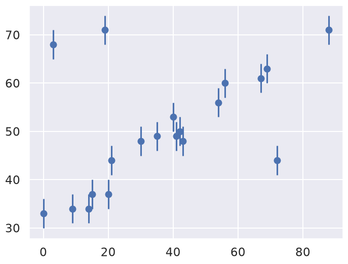
Our task is to find a line of best-fit to the data. It’s clear upon visual inspection that there are some outliers among these points, but how do we deal with them. In the subsequent sections we will consider both frequentist and Bayesian approaches. But first we need to set up our model.

The Model

Here we review the procedure for fitting a straight line to data, emphasizing the role of the statistical model. We take as our model (“\(M\)” here stands for “Model”; elsewhere we use “th” for theory),

\[ y_M(x; \boldsymbol{\theta}) = \theta_0 + \theta_1 x , \]

where our parameter vector will be

\[ \boldsymbol{\theta} = [\theta_0, \theta_1]. \]

But this is only half the picture: what we mean by a “model” in a Bayesian sense is not only this expected value \(y_M(x;\boldsymbol{\theta})\), but a probability distribution for our data. That is, we need an expression to compute the likelihood \(p(D\mid\boldsymbol{\theta},I)\) for our data as a function of the parameters \(\boldsymbol{\theta}\).

The Bayesian statistical model we employ is that the distribution of data \(D\) is the sum of the distributions for the model, the model discrepancy, and the observation error:

\[ D = M + \delta M + \delta D . \]

The model discrepancy term \(\delta M\) is in general important to consider, but we will neglect it here (e.g., assuming it is much smaller than \(\delta D\)).

To establish \(\delta D\), we note that here we are given data with simple error bars, which imply that the probability for any single data point is a normal distribution about the true value. In this example, the errors are specified by a single parameter \(\sigma_0\) (again, we neglect \(\delta M\)). That is, \(y_i = D_i\) is given by

\[ y_i \sim \mathcal{N}(y_M(x_i;\boldsymbol{\theta}), \sigma_0^2) \]

or, in functional form,

\[ p(y_i\mid x_i,\boldsymbol{\theta}) = \frac{1}{\sqrt{2\pi\sigma_0^2}} \exp\left(\frac{-\left[y_i - y_M(x_i;\boldsymbol{\theta})\right]^2}{2\sigma_0^2}\right) \]

The (known) variance of the measurement errors, \(\sigma_0\), is indicated in the figure below by the error bars.

Assuming all the points are independent, we can find the full likelihood by multiplying the individual likelihoods together:

\[ p(D\mid\boldsymbol{\theta}, I) = \prod_{i=1}^N p(y_i\mid x_i,\boldsymbol{\theta}, I) . \]

For convenience (and also for numerical accuracy) this is often expressed in terms of the log-likelihood:

(12.1)\[\begin{align} \log p(D\mid\boldsymbol{\theta}, I) &= -\frac{1}{2}\sum_{i=1}^N\left(\log(2\pi\sigma_0^2) + \frac{\left[ y_i - y_M(x_i;\theta)\right]^2}{\sigma_0^2}\right) \\ &= \text{constant} - \sum_{i=1}^N \frac{\left[ y_i - y_M(x_i;\boldsymbol{\theta})\right]^2}{2 \sigma_0^2} . \end{align}\]

We often define the residuals (the notation \(z_i\) is also common)

\[ R_i = \left[ y_i - y_M(x_i;\boldsymbol{\boldsymbol{\theta}}) \right]/\sigma_0, \]

so that the relevant chi-square sum is \(\chi^2 = \sum_{i=1}^N R_i^2\).

The summation term that appears in this log-likelihood is often known as the loss function. This particular loss function is known as a squared loss or chi-squared; but as you can see it can be derived from the Gaussian log likelihood.