4.3. Probability density functions

The key mathematical entity used over and over again throughout this book will be the “probability density function”, or just PDF for short. The PDF for continuous quantities can be integrated over a domain to obtain probabilities. An example familiar to every physicist will be the probability density of a quantum-mechanical particle. Max Born somewhat belatedly decided to put a square on Schrödinger’s wave function when interpreting the integral from \(x=a\) to \(x=b\) as the probability of measuring the particle to be between \(a\) and \(b\):

\[ \prob(a \leq x \leq b) = \int_a^b |\psi(x)|^2\, dx \]

We note that the unit of \(|\psi(x)|^2\) is inverse length, and it is generally true that PDFs, unlike probabilities, have units. If we divorce the previous equation from the quantum-mechanical context we would write:

\[ \prob(a \leq x \leq b) = \int_a^b \p{x}\, dx \]

where \(\p{x}\) is the PDF for the continuous variable \(x\).

Checkpoint question

What is the unit of \(p(\xvec)\) (or \(|\psi(\xvec)|^2\)) in three dimensions (assuming \(\xvec\) is a position vector measured in units of length)?

Answer

We can use the normalization equation (which is the sum rule):

\[ \int d^3x\, p(\xvec) = 1 , \]

which is dimensionless on the right side, so the unit of \(p(\xvec)\) (or \(|\psi(\xvec)|^2\)) is the inverse unit of \(d^3x\), or \(1/\text{length}^3\). Note that if \(\xvec\) represented a different quantity, the unit of \(p(\xvec)\) would differ accordingly.

We note that the case of a discrete random variable, e.g., the numbers that can be rolled on a die, mean that the PDF only is non-zero at a discrete set of allowed outcomes. In that case \(\p{x}\) can be represented as a sum of Dirac delta functions, and the resulting object is sometimes called a probability mass function (PMF). Thus the cases discussed above, in which \(\prob\) represented probability measured over a discrete set of outcomes, can be understood as special cases of PDFs.

In fact, working this from the other end, the sum and product rules for PDFs look just the same way as they do for probabilities. Therefore Bayes’ theorem (or rule) can also be applied to relate the PDF of \(x\) given \(y\), \(\pdf{x}{y}\) to the pdf of \(y\) given \(x\), \(\pdf{y}{x}\).

In Bayesian statistics there are PDFs (or PMFs if discrete) for everything. Here are a few examples:

• fit parameters — like the slope and intercept of a line in a straight-line fit

• experimental and theoretical imperfections that lead to uncertainties in the final result

• events (“Will it rain tomorrow?”)

We will stick to the \(\p{\cdot}\) notation here, but it’s worth pointing out that many different variants of the letter \(p\) are used to represent probabilities and PDFs in the literature. If we are interested in the PDF in a higher-dimensional space (say the probability of finding a particle in 3D space) you might see \(p(\vec x) = p(\mathbf{x}) = P(\vec x) = \text{pr}(\vec x) = \text{prob}(\vec x) = \ldots\).

Checkpoint question

What is the PDF \(\p{x}\) if we know definitely that \(x = x_0\) (i.e., the outcome is fixed)?

Answer

\(\p{x} = \delta(x-x_0)\quad\) [Note that \(\p(x)\) is normalized.]

Joint and marginal PDFs

\(\p{x_1, x_2}\) is the joint probability density of \(x_1\) and \(x_2\). In quantum mechanics the probability density \(|\Psi(x_1, x_2)|^2\) to find particle 1 at \(x_1\) and particle 2 at \(x_2\) is a joint probability density.

Checkpoint question

What is the probability to find particle 1 at \(x_1\) while particle 2 is anywhere?

Answer

\(\int_{-\infty}^{+\infty} |\psi(x_1, x_2)|^2\, dx_2\ \ \) or, more generally, integrated over the domain of \(x_2\).

This is a specific example of the marginalization rule, now in the PDF context, that we discussed the general form for probabilities above. The marginal probability density of \(x_1\) is the result when we marginalize the joint probability distribution over \(x_2\):

\[ \p{x_1} = \int \p{x_1, x_2} \,dx_2 . \]

So, in our quantum mechanical example, it’s the probability density we get when we just focus on particle 1, and don’t care about particle 2. Marginalizing in the Bayesian context means “integrating out” a parameter one is–at least temporarily–not interested in, to leave the focus on the PDF of other parameters. This can be particularly useful if there are “nuisance” parameters in the statistical model that are just indirectly influencing the quantity of interest. A specific example could be a parameter that account for the impact of defects in the measuring apparatus, but ultimately one is interested in the physics that cab be extracted with the imperfect apparatus.

Note

You may have noticed that we wrote \(\p{x_1}\) and \(\p{x_1, x_2}\) rather than \(\pdf{x_1}{I}\) and \(\pdf{x1,x2}{I}\), where “\(I\)” is information we know but do not specify explicitly. Our PDFs will always be contingent on some information, so we were really being sloppy by trying to be compact. (See The continuum limit for more careful versions of these equations.)

Bayes’ theorem applied to PDFs

The rules applied to probabilities in Section 4.2 directly extend to continuous functions, i.e., PDFs; we’ll summarize the extension briefly here. Conventionally we denote by \(\thetavec\) a vector of continuous parameters we seek to determine (for now we’ll use \(\alphavec\) as another vector of parameters). As before, information \(I\) is kept implicit.

Sum rule

Probabilities integrate to one (assuming exhaustive and exclusive \(\thetavec\)):

\[ \int d\thetavec\, \pdf{\thetavec}{I} = 1 . \]

The sum rule implies marginalization:

\[ p(\thetavec|I) = \int d\alphavec\, p(\thetavec, \alphavec | I) . \]

Product rule

Expanding a joint probability of \(\thetavec\) and \(\alphavec\)

(4.6)\[ p(\thetavec, \alphavec| I) = p(\thetavec | \alphavec, I) p(\alphavec,I) = p(\alphavec| \thetavec,I) p(\thetavec,I) . \]

As with discrete probabilities, there is a symmetry between the first and second equalities. If \(\thetavec\) and \(\alphavec\) are mutually independent, then \(p(\thetavec | \alphavec,I) = p(\thetavec | I)\) and

\[ p(\thetavec,\alphavec | I) = p(\thetavec|I) p(\alphavec | I) . \]

Rearranging the 2nd equality in (4.6) yields Bayes’ rule (or theorem) just like in the discrete case:

\[ p(\thetavec | \alphavec,I) = \frac{p(\alphavec|\thetavec,I) p(\thetavec|I)}{p(\alphavec | I)} \]

Bayes’ rule tells us how to reverse the conditional: \(p(\alphavec|\thetavec) \Rightarrow p(\thetavec|\alphavec)\). A typical application is when \(\alphavec\) is a vector of data \(\data\). Then Bayes’ rule is

\[ \overbrace{ \pdf{\thetavec}{\data,I)} }^{\textrm{posterior}} = \frac{ \color{red}{ \overbrace{ \pdf{\data}{\thetavec,I} }^{\textrm{likelihood}}} \color{black}{\ \times\ } \color{blue}{ \overbrace{ \pdf{\thetavec}{I}}^{\textrm{prior}}} } { \color{darkgreen}{ \underbrace{ \pdf{\data}{I} }_{\textrm{evidence}}} } \]

Viewing the prior as the initial information we have about \(\thetavec\) (i.e., before seeing the data \(\data\)), expressed as a PDF, then Bayes’ theorem tells us how to update that information after observing some data: this is the posterior PDF. In Section 6 we will give some examples of how this plays out when tossing biased coins.

Visualizing PDFs

Some visualizations of one-dimensional PDFs are shown here: a Gaussian (or normal) distribution; a Student t distribution (with overlaid normal distribution with the same standard deviation); two beta distributions with different parameters (the second one corresponds to a uniform distribution). The mode (maximum value), mean (average value), and median (50% of the probability is below and above) are shown for each distribution.

Show code cell source

Hide code cell source

import scipy.stats as stats  # We'll use stats as our source of PDFs
import numpy as np

import matplotlib.pyplot as plt
import corner  # for making "corner plots" showing 2-dimensional posteriors

import seaborn as sns; sns.set()  # nicer plots!

def dist_stuff(dist):
    """
    Finds the median, mean, and 68%/95% credible intervals for the given 
    1-d distribution (which is an object from scipy.stats).  
    """
    # For x = median, then mean: return x and the value of the pdf at x as a list
    median = [dist.median(), dist.pdf(dist.median())]  
    mean = [dist.mean(), dist.pdf(dist.mean())]
    # The left and right limits of the credibility interval are returned
    cred68 = dist.interval(0.68)  # 68% interval
    cred95 = dist.interval(0.95)  # 95% interval
    return median, mean, cred68, cred95

def dist_mode(dist, x):
    """
    Return the mode (maximum) of the 1-d distribution for array x. 
    """
    x_max_index = dist.pdf(x).argmax()
    # Return x of the maximum and the value of the pdf at that x 
    mode = [x[x_max_index], dist.pdf(x[x_max_index])]
    return mode

def dist_plot(ax, dist_label, x_dist, dist, color='blue'):
    """
    Plot the distribution, indicating median, mean, mode
    and 68%/95% probability intervals on the axis that is passed (ax).
    """
    median, mean, cred68, cred95 = dist_stuff(dist) 
    mode = dist_mode(dist, x_dist)
    
    plt.rcParams.update({'font.size': 20})  

    ax.plot(x_dist, dist.pdf(x_dist), label=dist_label, color=color)    
    ax.set_xlabel('x', fontsize=20)
    ax.set_ylabel('p(x)', fontsize=20)
    ax.tick_params(axis='both', which='major', labelsize=20)
    
    # Point to the median, mode, and mean with arrows (adjusting the spacing)
    text_x = 0.2*(x_dist[-1] - x_dist[0])
    text_x_mid = (x_dist[-1] + x_dist[0]) / 2.
    text_y = mode[1]*1.15
    ax.annotate('median', xy=median, xytext=(text_x_mid+text_x, text_y),
                arrowprops=dict(facecolor='black', shrink=0.05))
    ax.annotate('mode', xy=mode, xytext=(text_x_mid-text_x, text_y),
                arrowprops=dict(facecolor='red', shrink=0.05))
    ax.annotate('mean', xy=mean, xytext=(text_x_mid, text_y),
                arrowprops=dict(facecolor='blue', shrink=0.05))
    
    # Mark the credible intervals using shading (with appropriate alpha)
    ax.fill_between(x_dist, 0, dist.pdf(x_dist), 
                    where=((x_dist > cred68[0]) & (x_dist < cred68[1])), 
                    facecolor='blue', alpha=0.2)
    ax.fill_between(x_dist, 0, dist.pdf(x_dist), 
                    where=((x_dist > cred95[0]) & (x_dist < cred95[1])), 
                    facecolor='blue', alpha=0.1)
    
    ax.legend(fontsize=18);


# Make some standard plots: normal, beta
fig = plt.figure(figsize=(15,10))

# Standard normal distribution -- try changing the mean and std. dev. 
x_norm = np.linspace(-4, 6, 500) 
mu = 1       # mean
sigma = 2.0  # standard deviation
norm_dist = stats.norm(mu, sigma) # the normal distribution from scipy.stats
norm_label='normal pdf' + '\n' + rf'$\mu=${mu:1.1f}' \
             + '\n' + rf'$\sigma=${sigma:1.1f}' 
ax1 = fig.add_subplot(2,2,1)  # first of three subplots
dist_plot(ax1, norm_label, x_norm, norm_dist)

x_t = np.linspace(-5, 5, 500)
norm1_dist = stats.norm(0.,1.)  # a normal distribution for comparison

# plot of the Student t distribution
nu1 = 1.01
t1_dist = stats.t(nu1) # the Student t distribution
t1_label='t pdf' + '\n' + rf'$\nu=${nu1:1.1f}'
ax2 = fig.add_subplot(2,2,2)
dist_plot(ax2, t1_label, x_t, t1_dist)
ax2.plot(x_t, norm1_dist.pdf(x_t), color='red')

# beta distribution, characterized by a and b parameters
x_beta = np.linspace(-0.1, 1.1, 500)  # beta ranges from 0 to 1 
a1 = 2
b1 = 1
beta_dist = stats.beta(a1, b1)  # the beta distribution from scipy.stats
beta1_label='beta pdf' + '\n' + rf'$a=${a1:1.1f}' \
              + '\n' + rf'$b=${b1:1.1f}'
ax3 = fig.add_subplot(2,2,3)  # 
dist_plot(ax3, beta1_label, x_beta, beta_dist)

# another beta distribution
#x_beta = np.linspace(-0.1, 1.1, 500)
a2 = 1
b2 = 1
beta2_dist = stats.beta(a2, b2)
beta2_label='beta pdf' + '\n' + rf'$a=${a2:1.1f}' \
              + '\n' + rf'$b=${b2:1.1f}' 
ax4 = fig.add_subplot(2,2,4)  # 
dist_plot(ax4, beta2_label, x_beta, beta2_dist)

mu2 = beta2_dist.mean()
sigma2 = beta2_dist.std()
norm2_dist = stats.norm(mu2, sigma2)

fig.tight_layout()

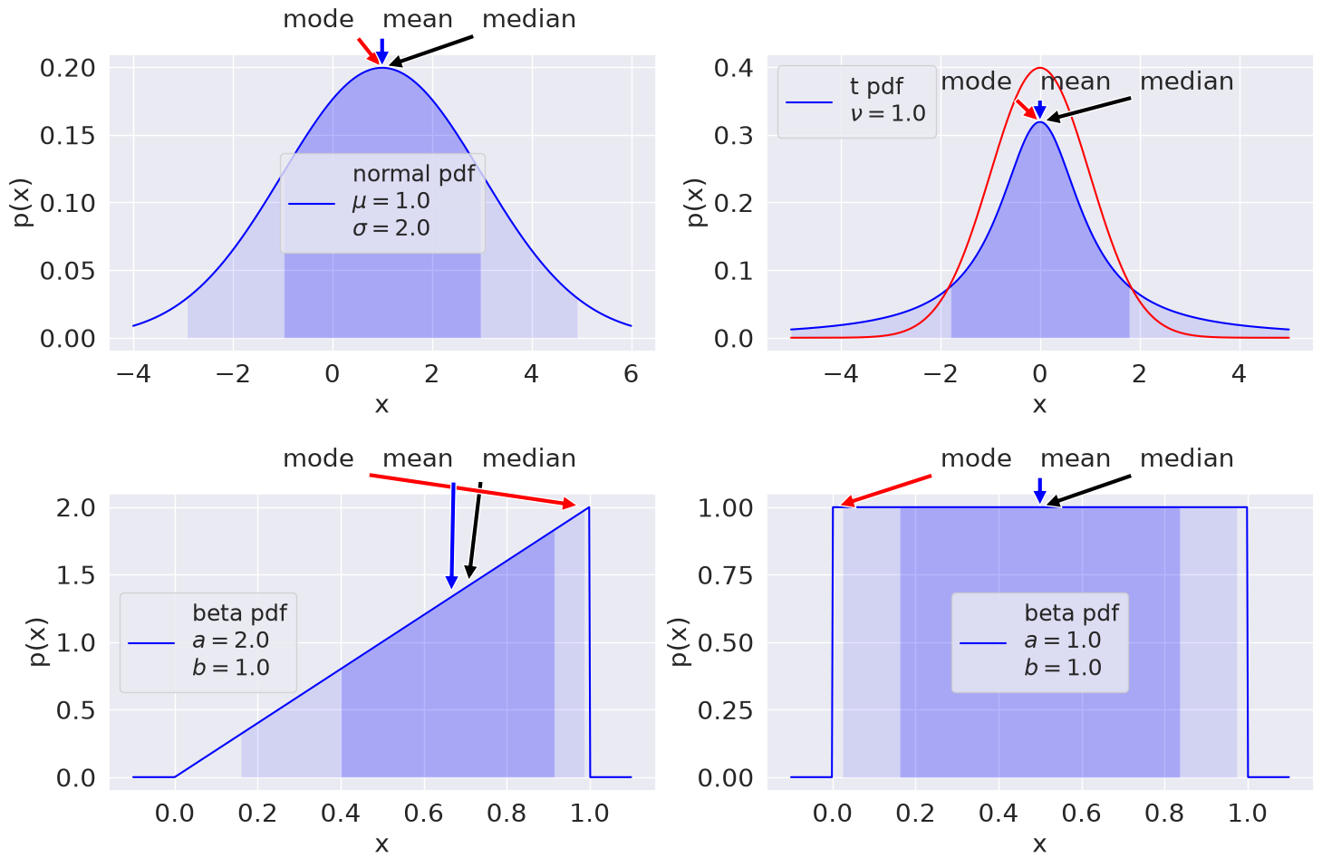
The 68%/95% probability regions are shown in dark/light shading. When applied to Bayesian posteriors, these are known as credible intervals or DoBs (degree of belief intervals). One can also encounter the name Bayesian confidence intervals, but this use of the label “confidence interval” is not recommended. The horizontal extent on the \(x\)-axis translates into the vertical extent of the error bar or error band for \(x\). The values of the mode, mean, median can be used as point estimates for the “probable” value of \(x\).

These examples are just a taste of a large range of standard distributions that are available in the python package scipy.stats. You can look at the code that generated the figures here (“Show code cell source”) but it may be worthwhile at this stage to jump ahead and explore using the demo notebook 📥 Demo: Exploring PDFs to make a hands-on pass at getting familiar with PDFs and how to visualize them using scipy.stats.

You can also get a preview of the effects of finite sampling. Since we can draw an arbitrary number of samples from the distributions defined in scipy.stats, we can see how the distributions build up as the number of samples increases, with decreasing fluctuations around the asymptotic distribution.

Note

See Statistics concepts and notation in Appendix A for further details on PDFs. You can also consult the scipy.stats manual page on statistical functions.

The diversity of available distributions should make it clear that the “default” choice of a Gaussian distribution is just that: a default choice. We will explore why this default choice is often the correct one in More on Gaussian distributions. But often is not the same as all the time, and it is frequently the case that another distribution gives a better description of the way data is distributed.

Trivia: Who was “Student”?

“Student” was the pen name of the Head Brewer at Guinness — a pioneer of small-sample experimental design (hence not necessarily Gaussian). His real name was William Sealy Gosset. “Statistics and Beer Day” is sometimes observed on his birthday, June 13, to celebrate his contributions.

Confidence intervals

Bayesian credible intervals: how are they defined?

Answer

The Bayesian credible interval for a parameter with a one-dimenional PDF is defined for a given percentage, call it \(\beta\%\). The interval is such that integrating over it one gets \(\beta\%\) of the total area under the PDF. The choice of interval is not unique. In particular, several reasonable intervals can be considered if the PDF is multimodal or skewed.

Point estimates

Various “point estimates” were introduced (mean, mode, median); which is “best” to use?

Answer

A point estimate is a one-number summary of a distribution. Which one is best to use depends on the application. Sometimes one wants to know the most likely case: then use the mode. Sometimes one really wants the average: then use the mean. Sometimes, for an asymmetric distribution, the median is the best estimate. For a symmetric, unimodal PDF, the three point estimates are the same. Note that to a Bayesian, a point estimate is only a rough approximation to the information in the full distribution.