
8.2. Bayesian research workflow#
The most common Bayesian analyses entail applications of Bayes’ rule:
To robustly construct the ingredients of Bayes’ rule and explore its consequences, we consider a four-step Bayesian workflow, first presented in Section 2.2 and repeated here:
Four-step Bayesian workflow in brief
Define a statistical model relating the physics model and data, including all errors and correlations.
Formulate priors.
Compute the posterior probabilities.
Do model checking.
In this chapter we elaborate on these steps. Our discussion is partially based on the more extensive exposition in the “Methods Primer” by Van De Schoot et al. [vandSchootDK+21]. (Note: discussion of how to use and calculate the evidence is postponed to Model Selection.)
These four main steps of a typical Bayesian workflow are indicated on the left in Fig. 8.7: (1) determine the likelihood function using information about the data generating process through a statistical model; (2) formulate prior distributions that embody knowledge about parameters in the statistical model (this step is conceptually performed before conditioning on data, and ideally, where practical, before those data are examined); (3) calculate the posterior distribution by using Bayes’ rule to combine the prior distribution and the likelihood function. The posterior distribution is then used to conduct inferences; (4) Use the posterior to check the extent to which aspects of the statistical model are consistent with the data being analyzed. While the four numbered steps provide a useful linear skeleton, the actual workflow consists of nested cycles and feedback.
In the following subsections we expand upon each step, detailing the cycles indicated on the right in Fig. 8.7.
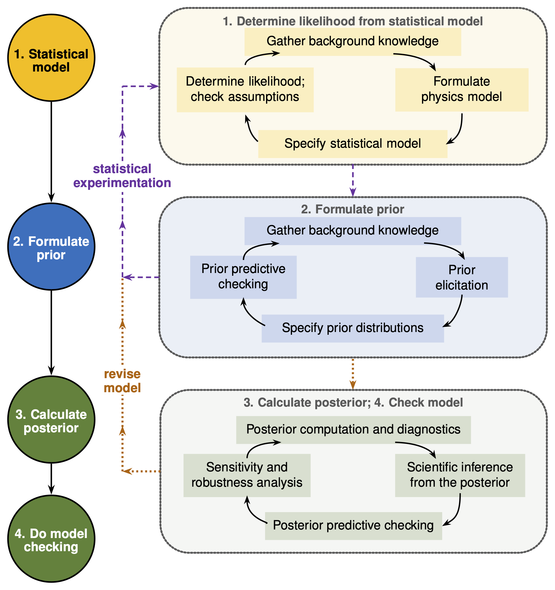
Fig. 8.7 The Bayesian research workflow. The workflow starts with specifying a data-generating statistical model and then determining the likelihood. The next step is formulating prior distributions. At this point the posterior distribution can be calculated from the product of the specified prior and likelihood function according to Bayes’ rule. Finally, there are checks to be made of the statistical model using that posterior. At each stage there is a cycle and the overall inferences that can be made can then be used to start a new research cycle. (Figure adapted from a diagram in [vandSchootDK+21] but note that the details and ordering of steps are different.)#
Step 1: Determining the likelihood#
The likelihood is common to both Bayesian and frequentist approaches, where it quantifies the degree to which observed data implies possible values for the unknown parameters. Since observed data is generated stochastically, through an underlying data-generating process, it is appropriately described by a probability distribution. This is the \(\text{``data likelihood''}\) that describes the probability distribution for observed data given a specific data-generating process (as indicated by the information on the right-hand side of the conditional).
The first step in formulating the data likelihood is to gather background knowledge and then formulate a physics model \(M(\pars)\), which relates the parameter(s) of interest to model outputs. A particular likelihood follows from a statistical model that stochastically generates the data; it incorporates the physics model, the data uncertainty \(\delta \data\), and the model discrepancy \(\delta M\). The additive statistical model from (4.11) combines these elements as random variables:
Assigning probability distributions and correlations to \(\delta \data\) and \(\delta M\) induces the data distribution \(\pdf{\data}{\thetavec,I}\). The statistical model should account for possible correlations in the outputs (type-y correlations). Such correlations result in a multivariate statistical distribution for the random variable \(\output\) that does not simply factor into a product of independent, univariate ones for each datum.
One can consider two views on the likelihood:
Generative view: Assuming specified values of \(\pars\), what possible data would the statistical model generate, and with what probabilities?
Likelihood view: Focusing on the observed data \(\data_\mathrm{obs}\) that we have; how does the likelihood for this data set depend on the values of the model parameters?
The first view is used for prior and posterior predictive simulation. The second view is the one that we adopt when allowing model parameters to be associated with probability distributions in Bayesian inference. The likelihood still describes the probability for observing a set of data, but we emphasize its parameter dependence by defining the likelihood function
Note that the likelihood function \(\mathcal{L}(\pars)\) is not a probability distribution for model parameters (and is not normalized, i.e., its integral over \(\pars\) is not equal to one). The parameter posterior regains status as a probability density for \(\pars\) through Bayes’ rule since the likelihood is multiplied with the prior \(\pdf{\pars}{I}\) and normalized by the evidence \(\pdf{\data}{I}\).
A product of normal distributions, one for each output, is a standard choice for a likelihood function. However, this choice assumes that the data generating process for one output is conditionally independent from the data generating process for any other output. In practice there may be correlations between them, e.g., shared analysis tools, electrical noise that is correlated between detectors, etc.
Just like the physics model and the prior, the statistical data-generating model is a modeling choice that needs to be justified, documented, and checked.
The latter may lead to revisiting the background knowledge and repeating the cycle in Step 1.
Step 2: Formulating and checking a prior#
The second major step in the Bayesian workflow depicted in Fig. 8.7 is to determine prior distributions, shortened to priors. This is an important part of a rigorous inference process. As we will discuss towards the end of our presentation of step 2, part of the cycle that occurs within this step is a prior predictive checking process (see Remark 8.1). This evaluates whether the priors chosen are doing the job they were designed to do. For this reason, prior selection, prior checking, and Step 1, Likelihood determination, are sometimes collectively referred to as the statistical experimentation phase.
Start with what you know#
Formulating the prior means encoding prior knowledge as a probability distribution. In this way pieces of information on the parameters of the model–or on other aspects of it–get included in the Bayesian analysis.
Sometimes the practitioner themselves has prior knowledge regarding parameters of the model. For example, a parameter may be known to be positive or otherwise strictly constrained by physics (e.g., causality). More broadly, almost all physics-model parameters have reasonable ranges, based on the mass, distance, and time scales appearing in the problem being analyzed. Order-of-magnitude estimates for parameters are completely valid fodder for priors, as long as the priors are chosen broadly enough to enable indications if the parameters are “unnatural”, i.e., out-of-line with those estimates.
Prior elicitation is the formal name for the process through which this kind of prior knowledge gets encoded in probability distributions. Prior elicitation may involve discussing with other modelers what “reasonable ranges” for parameters might be: “Would you be shocked if this parameter were smaller than…?”, “What is the order of magnitude of this parameter?”. People may sometimes say they have no idea what a parameter value would be, but they always have some idea!
If this process ultimately yields no, or very little, information on a parameter then priors can be assigned that reflect ignorance of its location or scale. The fact that the prior doesn’t depend on that parameter implies there is a symmetry or invariance principle that applies to the prior, and that principle can be employed to ensure the prior is consistent with the practitoner’s level of ignorance. See Section 11.1 for more on this topic and specific examples.
At the other extreme, sometimes highly constraining prior information comes from previous analyses of the model that used other data sets. In this case the hyperparameters for the prior could be derived from sample data or summary statistics of those previous analyses. However, this route to a prior must avoid “double-dipping”: the data used to form the prior needs to be distinct from the data included in the likelihood.
That’s because priors should encode background knowledge that the practitioner possesses which is independent of the data whose generation is modeled through the likelihood. The strength, or, conversely, uncertainty of that knowledge should be incorporated in the informativeness of the prior.
Critics of Bayesian methods often point to the subjectivity of priors as a major drawback. Two distinct points should be mentioned in this context. First, many elements of the estimation process are subjective in the sense that they may differ from modeler to modeler. Different reasonable people may make different reasonable choices not only for priors, but also for the likelihood, and certainly for the model itself. Second, many there are circumstances in physics for which informative priors are a well-justified and principled choice, e.g., the positivity bounds already mentioned or a situation in which a parameter’s distribution is quite well delineated by previous data.
Turn what you know into a pdf#
Priors can come in many different distributional forms, such as a normal, uniform or Poisson distribution, etc. The choice of distributional form for the prior (as needed for a full Bayesian analysis) typically involves extra assumptions. Say that you wish to assign to a model parameter a prior with a specific mean value and standard deviation. In this scenario you are still left with the choice between many different distributional forms that fulfill those constraints. Fortunately, arguments based on the maximum entropy principle can help translate a finite set of pieces of prior information into a probability distribution such that as little additional information as possible is smuggled into the prior. These ideas are presented in Section 11.2 The principle of maximum entropy.
But the most important thing about a prior is its level of informativeness. The information reflected in a prior distribution can range from total uncertainty to near certainty. The degree of (un)certainty that a prior encodes is typically described as informative, weakly informative, or diffuse.
The informativeness of a prior should be assessed relative to physically meaningful parameter scales and, ultimately, through the implications of the prior for observable quantities. It is also useful to compare the scale of the prior with the scale over which the likelihood can constrain the parameter. Good practical advice on choosing priors can be found in the Stan Prior Choice Recommendations compendium on github.
Finally, there is the question of how to formulate a prior in a multi-dimensional parameter space. For convenience, priors are often formulated for each parameter separately and then combined assuming independence, i.e., the prior \(\pdf{\para}{I}\) is taken to be the product of the one-dimensional prior pdfs for each individual parameter. However, if previous data or a theoretical argument indicates that two parameters should be correlated, then that correlation should be incorporated into the prior. Note that correlations derived from the data set being analyzed should not be incorporated into the prior. These will emerge from the posterior when it is formed from the prior and the likelihood. Building them into the prior right from the start of the analysis would be an example of the “double dipping” warned about above.
Checking prior implications#
One should always check prior implications to ensure that the prior is not much more restrictive (or much broader) than the background knowledge that is used to motivate it. This starts with checking that the scales of parameters (which may be physical observables) are consistent with what is known. Because Bayesian inference can be sensitive to poorly chosen priors, it is important to check whether the specified prior produces reasonable (not implausible) values for output quantities as well. Even in the absence of a data-generating distribution from a statistical model (see Step 1), one can draw samples from the prior \(\pdf{\thetavec}{I}\) and evaluate the physics model \(M(\thetavec)\) alone, looking to see whether substantial probability is placed on physically impossible or strongly implausible outputs. If so, that may already be a good reason to revisit the prior choice, particularly if the data-generation process is not going to remediate this problem, i.e., it’s not going to move substantial amounts of probability around.
The full prior predictive check (see Remark 8.1 below) is a more thorough assessment of the prior choice. The prior predictive distribution is the distribution of all possible data that could be generated given the prior, the statistical model for the data-generating process, and the physics model that relates the parameters of the model to the outputs. Thus, in the workflow diagram in Fig. 8.7, it comes at the end of the cycle in Step 2, before confronting new data, and it may carry one back to Step 1. It can’t be carried out absent a specified data-generating process. That’s because a full prior predictive check assesses whether the combination prior + model + data-generation yields outcomes that are compatible with background knowledge and with the range of data that could reasonably have been anticipated before the data being analyzed are used. The prior predictive distribution will often be broad, since it reflects uncertainty before conditioning on the new data, but it should not place substantial probability on outcomes that are already known to be physically impossible or scientifically implausible. Such behavior signals that one or more ingredients of the analysis—the prior, the physics model, or the assumed statistical relation between model outputs and data—should be reconsidered,as indicated by the return line to Step 1 in Fig. 8.7.
We emphasize that the check being conducted here is against output values that are clearly “out of range”, e.g., are significantly different than the expected size of the data. A prior predictive check absolutely does not mean that the practitioner should adjust the prior until its predictions agree with the particular data set that will subsequently enter the likelihood.
Once the prior and likeilhood have been combined and the posterior computed the sensitivity of the results to details of the chosen prior should be assessed as part of the model checking phase of the Bayesian workflow (Step 4). This is a very useful piece of the workflow: it can provide reassurance that all the choices you agonized over when formulating your prior ultimately don’t make a significant difference to the inference of the quantities you care about. Or, it can show how your prior choices are affecting the posterior, which does not invalidate your analysis, but does perhaps merit furhter investigation and certainly warrants reporting in your final research product.
Step 3: Results for the posterior–and other things of interest#
In the Bayesian Research Workflow, after defining the statistical model and the deriving the associated likelihood function, the next step is to combine the likelihood with the prior and use the resulting posterior to estimate the unknown parameters of the model.
In contrast, the frequentist framework as typically applied for model fitting focuses on the expected long-term outcomes of an experiment with the intent of producing a single point estimate for model parameters such as the maximum likelihood estimate and associated confidence interval. Within the Bayesian Research Workflow, probability distributions are assigned to the model parameters. Remember: in Bayesian statistics, the focus is on estimating the entire posterior distribution of the model parameters, even if this distribution is ultimately summarized with associated point estimates, such as the posterior mean or median, and a credible interval.
In these lecture notes, we frequently use Markov Chain Monte Carlo (MCMC) for posterior inference, see Overview of Part III: Sampling—although more advanced sampling algorithms are also discussed, see Section 22. MCMC has two basic outcomes from the Markov chain and Monte Carlo integration: a set of parameter values sampled according to the posterior distribution and an estimate of that distribution (and its statistics). A workflow for MCMC sampling is detailed in Section 21.1. We emphasize that posterior computation is not complete until the sampling quality and robustness has been checked with appropriate diagnostics (see Section 21.2).
MCMC is able to indirectly compute inferences on the posterior distribution by simulating different sets of parameters according to the product of the prior probability and the likelihood. This results in sets of values for the parameters \(\para\) (vectors in the multi-dimensional setting) that are obtained from the posterior distribution with frequencies that will correspond to the posterior distribution if the MCMC has converged. This can be achieved despite the fact that a Bayesian posterior obtained from a likelihood and a prior will typically be high-dimensional, not have a closed analytic form, and only be known up to a constant of proportionality. The samples of values of the parameters are then used to obtain empirical estimates of the posterior distribution of interest. It is often more difficult to obtain converged estimates of multivariate distributions, or of the form of low-probability tails. It is therefore sometimes more useful to focus on the marginal posterior distribution of each parameter, or pairs of parameters. These marginal distributions are defined by integrating out all but one or two of the parameters from the multi-dimensional posterior.
One important payoff of MCMC sampling is that any quantity of interest that is a function of the model parameters can also be obtained by computing the function over the set of MCMC samples. This then generates a set of samples for that quantity which can be analyzed via summary statistics, histograms, etc. If we are interested in multiple quantities that are functions of the parameters we can represent their multi-dimensional distribution as samples in this sense, and so determine not just summary statistics for each one, but also the correlations between these derived quantities.
Step 4: Model checking#
Because the statistical model specifies a probability distribution for possible data conditional on the parameters, posterior draws of the parameters can be propagated through the data-generating model to generate replicated or future data through the predictive posterior distribution (PPD). The PPD is the distribution that the model predicts for the model outputs that were measured, given the posterior inferred from those data. The PPD is our first example of Step 4 in the Bayesian Research Workflow.
Another important check is to assess prior sensitivity. In general a Bayesian analysis should be re-run several times, with different, reasonable, prior choices in order to assess how, and if so, where, the posterior is affected by those choices.
Remark 8.1 (Prior and posterior predictive checking)
Within steps Steps 2 and 4 of diagram Fig. 8.7 are two examples of predictive checks, for the prior and the posterior. The prior and posterior predictive checks use closely related simulation procedures, but they involve checking against different things and they answer different questions. Prior predictive checking examines the implications of the prior together with the generative model without any conditioning on (and really without any looking at) the new data. Posterior predictive checking asks whether the fitted model can reproduce scientifically relevant features of the observed data.
The prior predictive distribution is given formally by:
As implied by this formula, a prior predictive check is carried out in practice by sampling the parameters \(\para\) from the prior, then generating data according to the data model given those sampled parameters. This allows a check of how the probability mass of prior predictions is distributed, in particular whether there is significant prior mass concentrated in implausible regions of the parameter space. Note, however, that data sets simulated from the prior should not be compared to the actual data \(D\); instead examining if the simulated outputs take on extreme values will help diagnose priors that are too strong, too weak, poorly shaped, or poorly located.
The posterior predictive distribution is given formally by:
where the first pdf under the integral is defined by the statistical model that relates the future data \(y\) to \(M(\pars)\), i.e., (4.11). Note that it is conditioned on the observed data, unlike the prior predictive distribution. (We see that the prior predictive distribution (8.4) is just a special case of the posterior predictive distribution with no observed data.)
Posterior predictive checking works by simulating data sets based on the fitted model parameters according to (8.5) and then comparing (with appropriate statistics) this distribution to the original data set. For example, one could make histograms of the simulated and original data sets for a visual comparison. If the model is good, various summary statistics (e.g., the sample mean and variance) should be the same in the original and simulated data sets.
Prior predictive checks may motivate revisions of the prior or the generative model, leading back to an earlier step in the workflow, as indicated by the dashed return line in Fig. 8.7. Posterior predictive checks primarily diagnose deficiencies in the fitted model and may motivate revised model assumptions (dotted return line). They can also reveal sensitivity to the prior, but prior revisions after examining the data should be reported as part of a sensitivity analysis or become part of a subsequent research cycle.
The sensitivity of the posterior to the inclusion of different outputs in the likelihood is reflective of the information content of that observable. Sensitivity studies of the posterior based on simulated outputs for different future data is a branch of statistical inference known as experimental design. It can help determine which observable(s) to spend resources on measuring to improve the accuracy and precision of a desired inference.
Reproducibility#
To enable physics research to be verified and reproduced, proper reporting on statistics is crucial. In particular, not reporting the choice of priors is bad Bayesian practice. The naive use of priors has many pitfalls. Practitioners should record what was done and justify it as part of the research output. Specifying priors is a way of declaring to future readers of your work what information you considered known before you began your data analysis. Similarly, specification of the likelihood should be clear and complete, as already discussed above.
Overall, the Bayesian research workflow offers multiple opportunities to follow good scientific practices that facilitate reproducibility. To quote Van De Schoot et al. [vandSchootDK+21]: “Allowing others to assess the statistical methods and underlying data used in a study (by transparent reporting and making code & data available) can help with interpreting the study results, the assessment of the parameters of the methods used, and the detection & fixing of errors.” To which, we would add, it also helps practitioners generalize your work to their research application. But, as Van De Schoot et al. also point out “Reporting practices are not yet consistent in this regard across fields or even journals in individual fields.”
To enable reproducibility and allow other researchers to run Bayesian statistics on the same data with different parametrizations, priors, model assumptions, or likelihoods, it is important that the data and code used are properly documented and shared following what Van De Schoot et al. call the “FAIR principles”: findability, accessibility, interoperability and reusability [vandSchootDK+21]. Van De Schoot recommends, and we agree, that data and code should be:
Shared via a publicly accessible repository (e.g., on github or through Zenodo),
Given a persistent identifier such as a DOI
Tagged with appropriate metadata (which also enables appropriate citation).
For true accessibility, developing proper documentation for the software is essential. This includes README files with installation steps; a quickstart guide; testing methods (e.g., unit tests); licensing and how to cite the software. The code itself should adhere to best practices such as the use of descriptive variable and function names and standardized docstrings. All all of this implicitly assumes practitioners are using open-source software–if at all possible–so that barriers to replicating scientific results are lowered.
Making these choices enables transparency in the scientific process. Nany scientific journals now have guidelines that specify requirements like these for code and data sharing.
Checklists#
We end this chapter with two different recommended checklists for statistically sound Bayesian inference that incorporate many of the points made in this chapter. The first one (see Remark 8.2) has mainly natural science applications in mind.
Remark 8.2 (Checklist for statistically sound Bayesian inference)
Interact with the experts (i.e., statisticians, applied mathematicians).
Identify all sources of experimental and theoretical uncertainties in this process.
Formulate statistical models for those uncertainties.
Account for correlations in observables (type y) when formulating the likelihood.
Choose priors that are as informative as you consider reasonable, consistent with background knowledge; check their implications and assess sensitivity to reasonable alternatives.
Use model checking to assess the adequacy of the analysis and identify possible model deficiencies.
Note that this first checklist matches up quite well with the Bayesian workflow given at the start of this section.
The second checklist, labeled WAMBS (when to Worry and how to Avoid the Misuse of Bayesian Statistics), originates in work by statistics experts from a wide range of application areas [vandSchootDK+21]. Here we have condensed the recommendations of the original WAMBS checklist in regard to monitoring the MCMC convergence since we will provide more details on this in Part III.
Remark 8.3 (An adapted version of the WAMBS checklist)
Here we have adapted the WAMBS-v2 checklist, an updated version of the WAMBS (when to Worry and how to Avoid the Misuse of Bayesian Statistics) checklist. Adapted from [vandSchootDK+21].
Ensure the prior distributions and the model or likelihood are well understood (see checklist above).
Describe them thoroughly in your research output (article, analysis notebook, etc.).
Use prior predictive checking to assess whether the prior and generative model imply scientifically plausible data.
Check convergence of your MCMC chain. (See MCMC Workflow section.)
To assess the impact of informative priors, compare the posterior results with an analysis using diffuse priors. This comparison can facilitate a deeper understanding of the impact the informative priors have on findings.
Examine the sensitivity of your results to priors, especially multivariate priors. These priors can be particularly influential on the posterior, even with slight modifications to the hyperparameters.
It may also be worth testing different forms for the likelihood, in order to see what impact they have on the final results.
Report findings, including Bayesian interpretations. Take advantage of explaining and capturing the entire posterior rather than simply using point estimates. It may be helpful to examine the density at different quantiles to fully capture and understand the posterior distribution.
Ticking all the boxes of checklists such as these can be considered an aspirational goal for performing a truly rigorous statistical inference in science.