5.1. One-dimensional PDFs

To a Bayesian, everything is a PDF

As we noted in Section 4.3, physicists are used to dealing with PDFs as normalized wave functions squared. For a one-dimensional particle, the probability density at \(x\) is

\[ |\Psi(x)|^2 \Longrightarrow p(x) \]

The probability of finding \(x\) in some interval \(a \leq x \leq b\) is found by integration:

\[ \mathbb{P}(a \leq x \leq b) = \int_a^b |\Psi(x)|^2 \; dx \]

Just as with “Lagrangian” vs. “Lagrangian density”, physicists are not always careful when saying probability vs. probability density.

Physicists are also used to multidimensional normalized PDFs as wave functions squared, e.g. probability density for particle 1 at \(x_1\) and particle 2 at \(x_2\):

(5.1)\[ |\Psi(x_1, x_2)|^2 \Longrightarrow p(x_1,x_2) \equiv p(\textbf{x}) \quad \mbox{with}\quad \textbf{x} \equiv \{x_1,x_2\} \]

(Note that you will find alternative notation in the physics and statistics literature for generic PDFs: \(p(\textbf{x}) = P(\textbf{x}) = \textrm{pr}(\textbf{x}) = \textrm{prob}(\textbf{x}) = \ldots\) ) We will consider two-dimensional PDFs as in (5.1) in Section 5.2.

Some other vocabulary and definitions to remember

• \(p(x_1,x_2)\) is the joint probability density of \(x_1\) and \(x_2\).

• The marginal probability density of \(x_1\) is: \(p(x_1) = \int\! p(x_1,x_2)\,dx_2\). In quantum mechanics, this corresponds to the probability to find particle 1 at \(x_1\) and particle 2 anywhere; that is, \(\int\! |\Psi(x_1,x_2)|^2 dx_2\) (integrated over the full domain of \(x_2\), e.g., 0 to \(\infty\)).

• “Marginalizing” = “integrating out” (eliminates from the posterior the “nuisance parameters” whose value you don’t care about, at least not at that moment).

In Bayesian statistics there are PDFs (or PMFs if discrete) for experimental and theoretical uncertainties, model parameters, hyperparameters (what are those?), events (“Will it rain tomorrow?”), etc. Even if \(x\) has the definite value \(x_0\), we can represent this knowledge with a PDF \(p(x) = \delta(x-x_0)\).

Characteristics of PDFs

What are the characteristics (e.g., symmetry, heavy tails, …) of different PDFs: normal, beta, student t, \(\chi^2\), \(\ldots\)

Answer

Check these yourself! Note that the answers will often depend on the parameter values for the distribution. A Student t distribution may have “heavy tails” (meaning more probability in the tails than a Gaussian would have) for some parameter values but for others it approaches a normal distribution (so by definition no heavy tails).

Sampling

What does sampling mean?

Answer

To sample a given distribution is to draw values that represent it. The probability to draw a specific value is given by the distribution. In Bayesian inference one is most often sampling a posterior distribution.

Verifying sampling

How do you know if a distribution is correctly sampled?

Answer

One way is to look at the (normalized) histogram. If correctly sampled, this should approximate the distribution and the approximation should improve with more samples.

Widget for exploring common one-dimensional PDFs

Notes on the controls for the widget:

• Use the PDF pulldown menu to switch between some standard distributions.

• The parameters for each distribution can differ. See the SciPy Statistical functions page for function definitions that show how these parameters influence the shapes of the PDFs.

• When using the sliders, you can use the left and right keyboard arrows to make small adjustments.

• If the overlay normal with same mean/std checkbox is selected, a Gaussian distribution with the same mean and standard deviation as the current PDF will be superposed.

• Note that you can create more horizontal space for the widget by toggling the three-line icon at the top left of the page frame.

Invariant PDFs

Why do many of the PDFs appear unchanged when you change their parameters?

Answer

It is because the plots are autoscaled. If you are changing a location (loc) parameter (such as \(\mu\) for a normal PDF), this will just translate the PDF on the \(x\)-axis without changing the shape or the \(y\)-axis values. If you are changing a scale parameter (such as \(\sigma\) for a normal PDF), this will change both the \(y\)-axis values and the \(x\)-axis values without changing the shape.

Matching a Student’s t distribution to a normal distribution

When you switch to the Student’s t PDF and check overlay normal with same mean/std, a normal distribution is not seen. Why not?

Answer

When you first switch to the t distribution, the value of \(\nu\) is 2. For \(\nu\leq 2\), the variance of the distribution is infinite. So there is not a finite Gaussian PDF to draw! Try changing \(\nu\) to 2.01 (or anything higher) while the box is checked.

\(\chi^2\) distribution

Many physicists learn to judge whether a fit of a model to data is good or to pick out the best fitting model among several by evaluating the \(\chi^2\)/dof (dof = “degrees of freedom”) for a given model and comparing the result to one. Here \(\chi^2\) is the sum of the squares of the residuals (data minus model predictions) divided by variance of the error at each point:

\[ \chi^2 \equiv \sum_{i=1}^{N_{\text{data}}} \frac{\bigl(y_i - f(x_i;\hat\pars)\bigr)^2}{\sigma_i^2} , \]

where \(y_i\) is the \(i^{\text th}\) data point, \(f(x_i;\hat\pars)\) is the prediction of the model for that point using the best fit for the parameters, \(\hat\pars\), and \(\sigma_i\) is the error bar for that data point. The degrees-of-freedom (dof), often denoted by \(\nu\), is the number of data points minus number of fitted parameters:

\[ \nu = N_{\text{data}} - N_{\text{fit parameters}} . \]

The rule of thumb is generally that \(\chi^2/\text{dof} \gg 1\) means a poor fit and \(\chi^2/\text{dof} < 1\) indicates overfitting.

We will consider this from a Model selection perspective in Frequentist hypothesis testing in Chapter 14. Here we will just consider the nature of the \(\chi^2\) distribution.

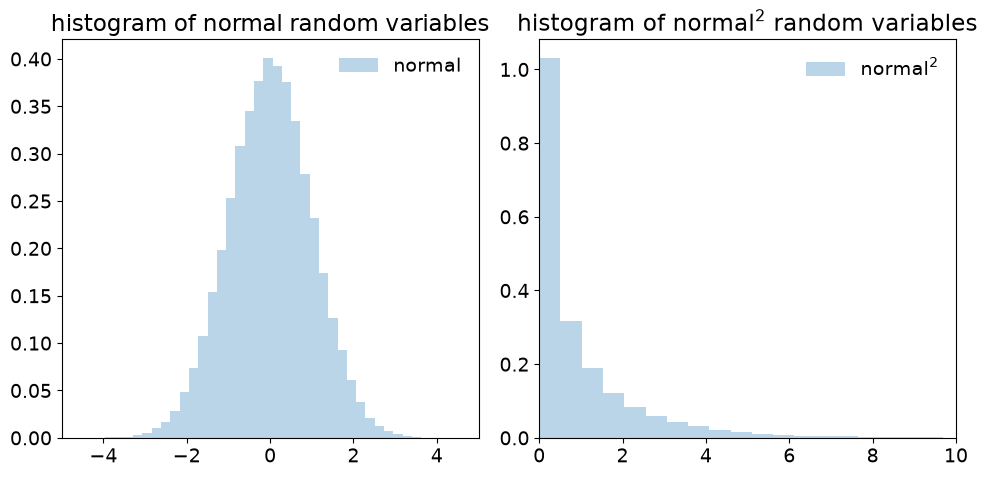
Test the sum of normal variables squared

The \(\chi^2\) distribution is supposed to result from the sum of the squares of Gaussian random variables. Here we test it numerically for two values of the degrees of freedom (dof). (You can try other cases by copying the code into a Jupyter notebook.) The Gaussian (normal) random variables are drawn from a standard normal distribution, i.e., with mean \(\mu = 0\) and \(\sigma = 1\).

Show code cell source

Hide code cell source

import numpy as np
import matplotlib.pyplot as plt
plt.rcParams.update({'font.size': 14})
import scipy.stats as stats

# sample tot_vals normal variables
tot_vals = 100000
x_norm_vals = stats.norm.rvs(size=tot_vals, random_state=None)

# plot a histogram of the normal variables and then their squares
fig, ax = plt.subplots(1, 2, figsize=(10,5))
ax[0].hist(x_norm_vals, bins=40, density=True, alpha=0.3, label='normal')
ax[0].set_xlim((-5, 5))
ax[0].legend(loc='best', frameon=False)
ax[0].set_title(fr'histogram of normal random variables')

ax[1].hist(x_norm_vals**2, bins=40, density=True, alpha=0.3, label=r'${\rm normal}^2$')
ax[1].legend(loc='best', frameon=False)
ax[1].set_title(fr'histogram of normal$^2$ random variables')
ax[1].set_xlim((0, 10))

fig.tight_layout()

def sum_norm_squares(num):
    """
    Return the sum of num random variables, with each the square of a random draw
    from a normal distribution
    """
    return np.sum(stats.norm.rvs(size=num, random_state=None)**2)

def histogram_per_dof(ax, num, x_min=0, x_max=5, tot_vals=1000):
    """
    Plot a histogram of sum of squares
      num --- number of squared normal-distributed random variables to sum
    """
    sum_xsq_vals = np.array([sum_norm_squares(num) for i in range(tot_vals)])
    scaled_sum = sum_xsq_vals/num
    ax.hist(scaled_sum, bins=40, density=True, alpha=0.3, 
        label='sum squares / dof')

    dofs = num
    x = np.linspace(0,5*dofs,1000)
    ax.plot(x/dofs, dofs*stats.chi2.pdf(x, dofs),
         'r-', lw=1, alpha=1, label=r'$\chi^2/dof$ PDF')

    ax.set_xlim((x_min, x_max))
    ax.legend(loc='best', frameon=False)
    ax.set_title(fr'$\chi^2/dof$ with dof = {dofs}')

    return ax

# Histograms per dof
tot_vals = 1000000  # no. of trials
fig, ax = plt.subplots(1, 2, figsize=(10,5))
num_lo = 5
ax[0] = histogram_per_dof(ax[0], num_lo, 0, 5)
num_hi = 100
ax[1] = histogram_per_dof(ax[1], num_hi, 0, 2)

fig.tight_layout()

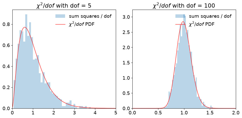
Check whether the distributions (which are of \(\chi^2/\nu\)) are consistent with the statement above that the mean of a \(\chi^2\) distribution with \(k = \nu\) dofs is \(\nu\), with variance \(2\nu\).

The near ubiquity of Gaussians

We will see a lot of Gaussian distributions in this course. Some people implicitly always assume Gaussian distributions. So this seems like a good place to pause and consider why Gaussian distributions are such a common choice. It turns out there are several reasons why one might choose a Gaussian to describe a probability distribution. Our first reason is closely related to the observation that leads to small amplitude oscillations in mechanics being harmonic. We will encounter two more reasons in The Central Limit Theorem and The principle of maximum entropy.

The Gaussian is to statistics what the harmonic oscillator is to mechanics

Suppose we have a probability distribution \(p(x | D,I)\) that is unimodal (has only one hump), then one way to form a “best estimate’’ for the variable \(x\) is to compute the maximum of the distribution. (To save writing we denote the PDF of interest as \(p(x)\) for a while hereafter.)

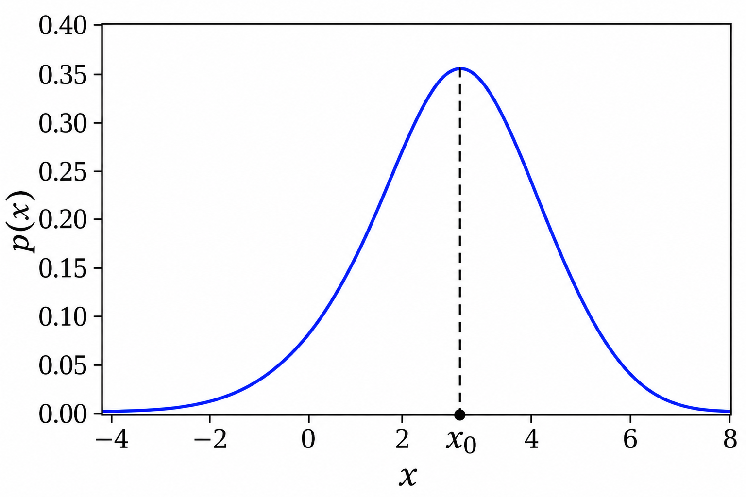
We find this point, which we’ll denote by \(x_0\), using calculus:

\[ \left.\frac{dp}{dx}\right|_{x=x_0} = 0 \quad \mbox{with} \quad \left.\frac{d^2p}{dx^2}\right|_{x=x_0} < 0 \ \text{(maximum)}. \]

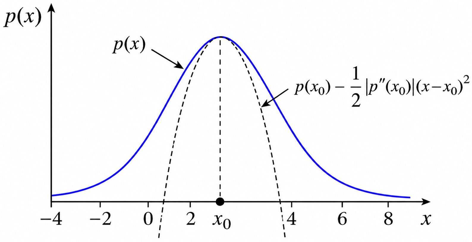
To characterize the posterior \(p(x)\), we look nearby. We want to know how sharp this maximum is: is \(p(x)\) sharply peaked around \(x=x_0\) or is the maximum kind-of shallow? To work this out we’ll do a Taylor expansion around \(x=x_0\). The PDF \(p(x)\) itself varies very rapidly, but since \(p(x)\) is positive definite we can Taylor expand \(\log p\) instead. (See the box below on “\(p\) or \(\log p\)?” for a strict mathematical reason why it’s problematic for our purposes to directly Taylor expand \(p(x)\) around its maximum.)

\[ \Longrightarrow\ L(x) \equiv \log p(x) = L(x_0) + \left.\frac{dL}{dx}\right|_{x = x_0}(x-x_0) + \frac{1}{2} \left.\frac{d^2L}{dx^2}\right|_{x = x_0}(x-x_0)^2 + \cdots \]

Note that \(\left.\frac{dL}{dx}\right|_{x = x_0}=0\), because \(L(x_0)\) is a maximum if \(p(x_0)\) is, and \(\left.\frac{d^2L}{dx^2}\right|_{x = x_0} < 0\). If we can neglect higher-order terms, then when we re-exponentiate,

\[ p(x) \approx A\, e^{\frac{1}{2}\left.\frac{d^2L}{dx^2}\right|_{x = x_0}(x-x_0)^2} , \]

with \(A\) a normalization factor that originates in the \(L(x_0)\) term. So in this general circumstance we get a Gaussian distribution:

\[ p(x) = \frac{1}{\sqrt{2\pi\sigma^2}}e^{-(x-\mu)^2/\sigma^2} \quad\Longrightarrow\quad \mu = x_0, \ \sigma = \left(-\left.\frac{d^2L}{dx^2}\right|_{x=x_0}\right)^{-1/2}, \]

where we see the importance of the second derivative being negative.

We usually characterize the distribution by \(x_0 \pm \sigma\) (e.g., with a point and symmetric error bars if this is data noise), because if it is a Gaussian this is sufficient to tell us the entire distribution. E.g., \(n\) standard deviations is \(n\times \sigma\). But for a Bayesian, the full posterior \(p(x|D,I)\) for all \(x\) is the general result, and \(x = x_0 \pm \sigma\) may be only an approximate characterization.

To think about …

What if \(p(x)\) is asymmetric? What if it is multimodal?

\(p\) or \(\log p\)?

We motivated Gaussian approximations from a Taylor expansion to quadratic order of the logarithm of a PDF. What would go wrong if we directly expanded the PDF? Well, if we do that we get:

\[ p(x) \approx p(x_0) + \frac{1}{2}\left.\frac{d^2p}{dx^2}\right|_{x=x_0}(x-x_0)^2 \ \overset{x\pm\rightarrow\infty}{\longrightarrow} -\infty, \]

i.e., we get something that diverges as \(x\) tends to either plus or minus infinity.

A PDF must be normalizable and positive definite, so this approximation violates these conditions!