21.5. Slice sampling#
The idea of slice sampling is well documented in
two arXiv references for the ensemble slice sampler zeus (which is a particular implementation):
Ensemble Slice Sampling: Parallel, black-box and gradient-free inference for correlated & multimodal distributions by Minas Karamanis and Florian Beutler.
zeus: A Python implementation of Ensemble Slice Sampling for efficient Bayesian parameter inference by Minas Karamanis, Florian Beutler, and John A. Peacock.
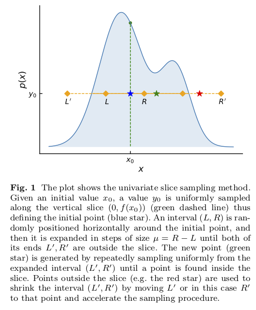
Slice sampling in action for a one-dimensional distribution is shown in Fig. 21.2. The idea is that sampling from a distribution \(p(x)\) is the same as uniform sampling from the area under the plot of \(f(x) \propto p(x)\). E.g., the highest probability \(p(x)\) is where the area is largest, and this is a simple proportionality. The height \(y\) is introduced with \(0 < y < f(x)\) as an auxiliary variable and one samples the uniform joint probability \(p(x,y)\). Then \(p(x)\) is obtained by marginalizing over \(y\) (meaning just dropping \(y\) from the sample).
The blue star comes from uniformly sampling in \(y\) at the initial point \(x_0\) to identify \(y_0\). The “slice” is the set of \(x\) such that \(y_0 < f(x)\). In the figure the interval initially from \(L\) to \(R\) is expanded to \(L'\) to \(R'\), which includes the full slice. When the final interval is found, a new \(x_1\) is drawn uniformly from the intersection of the interval and the slice.
The green star is an accepted new point \(x_1\) (inside the slice) while the red star is a rejected point (outside the slice).
There is one parameter to tune: the width \(\mu\) of the interval from \(L\) to \(R\) that sets the original interval around \(x_0\) and then the step size for expanding the interval to be from \(L'\) to \(R'\). In zeus the value of \(\mu\) is tuned by stochastic optimization.
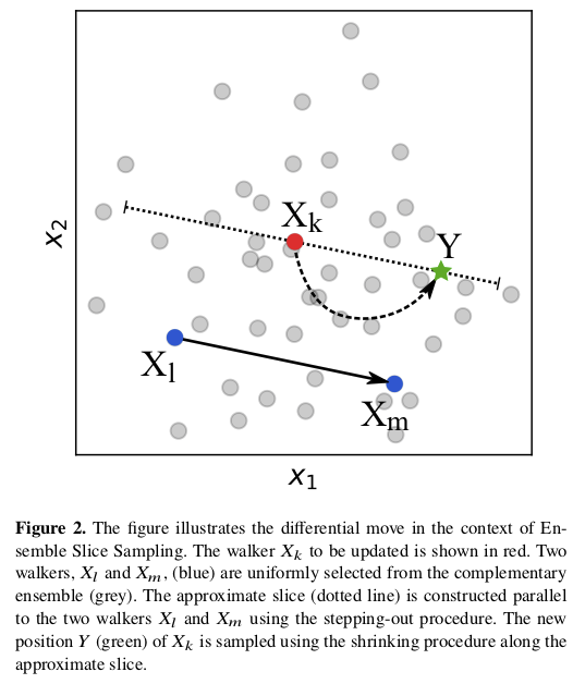
The “ensemble” aspect of zeus is that there are multiple walkers, as in the ensemble sampler emcee.
Fig. 21.3 illustrates how the ensemble of walkers is used to do what is called a “differential move”. There are several choices for moves, including a global one that is effective for multi-modal distributions.
A text case for parallel tempering (using
ptemcee) vs. slice sampling (usingzeus) in a very simple multi-modal example is in Demo: Multimodal distributions with the ptemcee and zeus samplers.The basic call for
zeuscompared toemceeandPyMCis illustrated in Comparing samplers for a simple problem.