7.1. Nuisance parameters and marginalization

The Bayesian approach offers a straightforward approach for dealing with (known) systematic uncertainties; namely by marginalization.

For example, assume that we have a model with two parameters, \(\theta\) and \(\phi\), although only one of them (say \(\theta\)) is of physical relevance. The other one is then labeled a nuisance parameter. If through a Bayesian data analysis we get the joint posterior PDF

(7.1)\[\begin{equation} \pdf{\theta, \phi}{\data, I}, \end{equation}\]

then the marginal posterior PDF \(\pdf{\theta}{\data, I}\) is obtained via marginalization

(7.2)\[\begin{equation} \pdf{\theta}{\data, I} = \int \pdf{\theta, \phi}{\data, I} \,d\phi. \end{equation}\]

Thus we have directly derived how to propagate the uncertainty in \(\phi\) to the probability distribution for \(\theta\).

Example 7.2 provides an illustration of this scenario.

Marginalization using samples

Assume that we have \(N\) samples from the joint pdf \(\pdf{\theta, \phi}{\data, I}\). This might be a sample chain from an MCMC sampler: \(\left\{ (\theta, \phi)_i \right\}_{i=0}^{N-1}\). Think of this as two columns of length \(N\). Then the marginal distribution of \(\theta\) will be given by the same chain by simply ignoring the \(\phi\) column, i.e., \(\left\{ \theta_{i} \right\}_{i=0}^{N-1}\).

See the Visualizations of MCMC created by Chi Feng for an illustration of this. In these simulations, the marginalization is performed by projecting the joint samples into a histogram on the \(x\) or \(y\) axis.

A slightly more general scenario for which the marginalization procedure is used for error propagation is the following: Assume that we have measured or inferred distributions for the random variables \(X\) and \(Y\); what can we say about the distributions for the difference \(X-Y\) or the raio \(X/Y\), or the sum of their squares \(X^2+Y^2\), etc?

Such questions can be rephrased as: Given the joint PDF \(\pdf{x,y}{I}\), what is \(\pdf{z}{I}\), where \(z=f(x,y)\)? In this situation we can use marginalization and the product rule.

(7.3)\[\begin{equation} \pdf{z}{I} = \int \pdf{z,x,y}{I}\,dx\,dy = \int \pdf{z}{x,y,I}\, \pdf{x,y}{I}\,dx\,dy. \end{equation}\]

We first realize that \(\pdf{z}{x,y,I} = \delta(z-f(x,y))\) due to the deterministic functional relationship between the parameters.

The joint PDF for \(X\) and \(Y\) becomes a product if the errors are independent \(\pdf{x,y}{I} = \pdf{x}{I} \pdf{y}{I}\) . Then the delta function can be used to evaluate one of the integrals, giving some inverse transformation \(y=g(x,z)\), and the PDF for \(Z\) becomes a convolution

(7.4)\[ \pdf{z}{I} = \int \pdf{x}{I}\, \pdf{y=g(x,z)}{I}\,dx. \]

Example 7.1 (\(Z = X + Y\))

Let us consider the situation where you are interested in the quantity \(Z = X + Y\), and you know that \(X\) and \(Y\) are distributed as independent Gaussians with \(\expect{X} = x_0\), \(\var{X} = \sigma_x^2\) and \(\expect{Y} = y_0\), \(\var{Y} = \sigma_y^2\). Then

(7.5)\[\begin{align} \pdf{x,y}{I} &= \pdf{x}{I}\,\pdf{y}{I} \\ &= \frac{1}{2\pi\sigma_x\sigma_y} \exp\left[ - \frac{(x-x_0)^2}{2\sigma_x^2} \right] \exp\left[ - \frac{(y-y_0)^2}{2\sigma_y^2} \right]. \end{align}\]

Let us now use marginalization and the product rule to find

(7.6)\[\begin{equation} \pdf{z}{I} = \int \pdf{z,x,y}{I}\,dx\,dy = \int \pdf{z}{x,y,I}\, \pdf{x,y}{I}\,dx\,dy. \end{equation}\]

We realize that \(\pdf{z}{x,y,I} = \delta(z-(x+y))\) due to the functional relationship between the random variables, and we have \(\pdf{x,y}{I}\) as a product of Gaussian PDFs from above. The delta function can be used to evaluate one of the integrals, and the PDF for \(Z\) becomes a convolution

(7.7)\[\begin{align} \pdf{z}{I} &= \int \pdf{x}{I}\, \pdf{y=z-x}{I}\, dx \\ &= \frac{1}{2\pi\sigma_x\sigma_y} \int \exp\left[ - \frac{(x-x_0)^2}{2\sigma_x^2} \right] \exp\left[ - \frac{(z - x - y_0)^2}{2\sigma_y^2} \right] dx. \end{align}\]

After some algebra that involves completing the square for \(X\) in the exponent we obtain

(7.8)\[ \pdf{z}{I} = \frac{1}{\sqrt{2\pi}\sigma_z} \exp\left[ - \frac{(z-z_0)^2}{2\sigma_z^2} \right], \]

with \(z_0 = x_0 + y_0\) and \(\sigma_z^2 = \sigma_x^2 + \sigma_y^2\). Thus, the PDF for the sum \(Z=X+Y\), with \(X\) and \(Y\) being described by Gaussian PDFs, is another Gaussian, with the uncertainties “adding in quadrature”.

Exercise 7.1 (Correlated errors)

For correlated errors, the joint PDF \(\pdf{x,y}{I}\) does not factorize into a product. Consider, for example, a situation with a bivariate normal distribution

\[ \pdf{x,y}{I} = \frac{1}{(2\pi) |\boldsymbol{\Sigma}|^{1/2}} \exp{ \left( -\frac{1}{2}(x, y)\boldsymbol{\Sigma}^{-1}(x, y)^T\right)}. \]

Furthermore, let us assume that the variances in \(X\) and \(Y\) are the same (\(\sigma_x^2=\sigma_y^2\equiv\sigma^2\)) and the covariance is positive and almost as large as the variance (i.e., errors are strongly correlated). Then, the linear transformation \(S=(X-Y)/\sqrt{2}\) and \(T=(X+Y)/\sqrt{2}\) gives two new random variables \(S\) and \(T\) that turn out to be independent. This implies

\[\begin{split} \pdf{x,y}{I} = \left\{ \begin{array}{l} s = \frac{x-y}{\sqrt{2}} \\ t = \frac{x+y}{\sqrt{2}} \\ \end{array} \right\} = \frac{1}{\sqrt{2\pi}\sigma_s}\exp \left( - \frac{s^2}{2\sigma_s^2} \right) \frac{1}{\sqrt{2\pi}\sigma_t}\exp \left( - \frac{t^2}{2\sigma_t^2} \right). \end{split}\]

Furthermore, given the strong positive correlation one finds that \(\sigma_s \ll \sigma\). What is the PDF for the difference \(Z=X-Y\) in this situation?

Exercise 7.2 (Sum of two Gaussian PDFs)

Complete the derivation of Eq. (7.8).

Example 7.2 (Inferring galactic distances)

The Hubble constant \(H\) acts as a galactic ruler as it is used to measure astronomical distances (\(d\)) according to \(v = H d\), where \(v\) is the velocity that can be measured with observations of redshifts. An error in \(H\) will therefore correspond to a systematic uncertainty in such measurements.

A modern value for the Hubble constant is \(H = 70 \pm 10\) km s\(^{-1}\) MPc\(^{-1}\). We introduce the expectation value \(\expect{H} = H_0 = 70\) km s\(^{-1}\) MPc\(^{-1}\) and the standard deviation \(\std{H} = \sigma_H = 10\) km s\(^{-1}\) MPc\(^{-1}\). Note that astronomical distances are usually measured in million parsecs (MPc). Suppose that a specific galaxy has a measured recessional velocity \(v_0 = 100 \times 10^3\) km/s with an observational error quantified by a standard deviation \(\sigma_v = 5 \times 10^3\) km/s. Determine the posterior PDF for the distance to a galaxy under the following three different analysis assumptions:

1. We use the expectation value of \(H\) in the analysis: \(H = H_0 = 70\) km s\(^{-1}\) MPc\(^{-1}\).

2. We include the uncertainty in the value of the Hubble constant via a Gaussian PDF:

   \[ \pdf{H}{I} = \frac{1}{\sqrt{2\pi}\sigma_H} \exp\left( - \frac{(H-H_0)^2}{2 \sigma_H^2} \right). \]

3. We include the uncertainty in the value of the Hubble constant via a uniform PDF:

   \[\begin{split} \pdf{H}{I} = \left\{ \begin{array}{ll} \frac{1}{4 \sigma_H} & \text{for } H_0 - 2\sigma_H \leq H \leq H_0 + 2\sigma_H, \\ 0 & \text{otherwise.} \end{array} \right. \end{split}\]

In addition, an approximate propagation of errors will be demonstrated in Section 7.3 in Example 7.3.

Here we use marginalization to obtain the desired posterior PDF \(\pdf{d}{\data,I}\) from the joint distribution of \(\pdf{d,H}{\data,I}\)

(7.9)\[ \pdf{d}{\data,I} = \int_{-\infty}^\infty \pdf{d,H}{\data,I} dH . \]

Using

• Bayes’ rule: \(\pdf{d,H}{\data,I} \propto \pdf{\data}{d,H,I} \pdf{d,H}{I}\),

• the product rule: \(\pdf{d,H}{I} = p(H|d,I)\pdf{d}{I}\),

• and the fact that \(H\) is independent of \(d\): \(p(H|d,I) = \pdf{H}{I}\),

we find that

(7.10)\[\begin{equation} \pdf{d}{\data,I} \propto \pdf{d}{I} \int \pdf{H}{I}\, \pdf{\data}{d,H,I}\, dH , \end{equation}\]

which means that we have expressed the quantity that we want (the posterior of \(d\)) in terms of quantities that we can specify, as follows.

First, we need to state our prior knowledge concerning the distance \(\pdf{d}{I}\). You might ask yourself what information is contained in this quantity. It should summarize our state of knowledge before accumulating the new data. For starters, we do know that it is a distance (meaning that it is a positive quantity) and we would also expect it to be smaller than the (visible) size of the universe. We might argue that it should be at least as far away as the previously known closest galaxy. Further arguments can be made on the basis of indifference, but we will defer such discussions for now. For simplicity, we just assign a uniform PDF

\[ \pdf{d}{I} \propto 1, \]

within some huge range \(0 < d < 10^9\) MPc.

The likelihood for the observed can be written down from a statistical model

\[ v_\mathrm{measured} = H d + \delta\mathcal{D}, \]

where \(H d\) represents our model for the velocity and \(\delta\mathcal{D}\) is the observational error, which is a random variable. We know that \(\expect{v_\mathrm{measured}} = v_0\) and \(\text{Var}(v_\mathrm{measured}) = \sigma_v^2\). Given this information it is motivated to use a Gaussian PDF (with this mean and variance) for the likelihood

\[ \pdf{\data}{d,H,I} = \frac{1}{\sqrt{2\pi}\sigma_v} \exp\left( - \frac{(v_0 - Hd)^2}{2\sigma_v^2} \right). \]

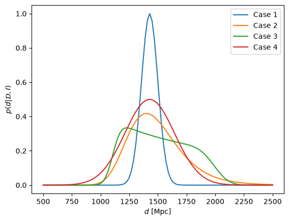
The results for the different analysis strategies (1-3 in the list above) should be obtained in Exercise 7.3. A comparison figure that also includes the approximate error propagation from Example 7.3 is shown in the solution to this exercise.

Exercise 7.3 (Inferring galactic distances)

Apply the three analysis strategies and derive the posterior distribution \(\pdf{d}{\data,I}\). The first case allows an analytical solution while the second and third are probably best approached numerically (although it is, in fact, possible to find an analytical result also for case 2). Plot the results.

Hint 1: Since the goal is to extract a probability distribution, and we are already ignoring the denominator in Bayes’ theorem, it is allowed to ignore all normalization constants. The final PDFs can be normalized by integration.

Hint 2: A fixed value for \(H\) can be assigned with the PDF \(\pdf{H}{I} = \delta(H-H_0)\), where \(\delta(x)\) is the Dirac delta function.

Solutions to exercises

Solution to Exercise 7.1 (Correlated errors)

\[\begin{align*} \pdf{z}{I} &= \int \pdf{z}{x,y,I}\, \pdf{x,y}{I}\, dx\,dy = \int \delta(z-\sqrt{2}s) p(s|I) p(t|I)\, ds\,dt \\ &= \left\{ \begin{array}{l} \tilde{s}=\sqrt{2}s \, \Rightarrow \, ds = d\tilde{s}/\sqrt{2} \\ \delta(z-\sqrt{2}s) \to \delta(z/\sqrt{2}-\tilde{s}) \end{array} \right\} = \frac{1}{\sqrt{2}\sqrt{2\pi}\sigma_s}\exp \left( - \frac{z^2}{4\sigma_s^2} \right) \int p(t|I)\, dt . \end{align*}\]

Here we can use that \(\int p(t|I)\, dt = 1\). Defining \(\sigma_z = \sqrt{2}\sigma_s\) we find

\[ \pdf{z}{I} = \frac{1}{\sqrt{2\pi}\sigma_z}\exp \left( - \frac{z^2}{2\sigma_z^2} \right) , \]

i.e. a normal distribution for \(z\) with a small variance \(2\sigma_s^2\).

Solution to Exercise 7.3 (Inferring galactic distances)

1. A fixed value for \(H\) can be assigned with the PDF \(\pdf{H}{I} = \delta(H-H_0)\), where \(\delta(x)\) is the Dirac delta function. We note that integrals over a delta function are given by \(\int_{-\infty}^{+\infty} f(x) \delta(x-x_0)\, dx = f(x_0)\) such that

   \[ \pdf{d}{\data,I} \propto \exp\left( - \frac{(v_0 - H_0 d)^2}{2\sigma_v^2} \right), \]

   where we have ignored all normalization coefficients.

2. With a Gaussian prior for \(H\) we will be left with an integral

   \[ \pdf{d}{\data,I} \propto \int_{-\infty}^{+\infty} dH\, \exp\left( - \frac{(H-H_0)^2}{2 \sigma_H^2} \right) \exp\left( - \frac{(v_0 - H d)^2}{2\sigma_v^2} \right). \]

   We can perform this integral numerically, or we can solve it analytically by realizing that the product of two Gaussian distributions is another Gaussian distribution.

3. The uniform prior for \(\pdf{H}{I}\) implies that the final integral becomes

   \[ \pdf{d}{\data,I} \propto \int_{H_0 - 2\sigma_H}^{H_0 + 2\sigma_H} dH \exp\left( - \frac{(v_0 - H d)^2}{2\sigma_v^2} \right). \]

For numerical integration, and plots of the results of the three inference strategies, see the hidden code block below.

Show code cell content

Hide code cell content

# Common imports
import numpy as np
import matplotlib.pyplot as plt
import scipy.integrate as integrate

# Given information
H0=70
sigH=10
v0=10**5
sigv=5000

# grid for evaluating and plotting p(d|...)
dgrid = np.linspace(500,2500,100)

# Case 1
def pdf_1(d):
    return np.exp(-(v0-H0*d)**2/(2*sigv**2))
# Case 2
def pdf_2(H,d):
    return np.exp(-(H-H0)**2 / (2*sigH**2)) * np.exp(-(v0-H*d)**2 / (2*sigv**2))
# ... with numerical integration over H
pdf_2_grid = np.zeros_like(dgrid)
for i_d,di in enumerate(dgrid):
  I = integrate.quad(pdf_2, 0, 140, args=(di))
  pdf_2_grid[i_d] = I[0] / 20
# Case 3
def pdf_3(H,d):
    return np.exp(-(v0-H*d)**2 / (2*sigv**2))
# ... with numerical integration
pdf_3_grid = np.zeros_like(dgrid)
deltaH = np.sqrt(12*sigH**2/4)
for i_d,di in enumerate(dgrid):
  I = integrate.quad(pdf_3, H0-2*sigH, H0+2*sigH, args=(di))
  pdf_3_grid[i_d] = I[0] / 30
# Case 4 (see example 9.3)
d0 = v0/H0
sigd = d0*np.sqrt(sigH**2/H0**2 + sigv**2/v0**2)
def pdf_4(d):
    return np.exp(-(d-d0)**2 / (2*sigd**2)) / 2
    
fig,ax = plt.subplots(1,1)
ax.plot(dgrid,pdf_1(dgrid),label='Case 1')
ax.plot(dgrid,pdf_2_grid,label='Case 2')
ax.plot(dgrid,pdf_3_grid,label='Case 3')
ax.plot(dgrid,pdf_4(dgrid),label='Case 4')

ax.set_xlabel(r'$d$ [Mpc]')
ax.set_ylabel(r'$p(d|\mathcal{D},I)$')
ax.legend(loc='best');