More on Gaussian distributions

5.3. More on Gaussian distributions#

The near ubiquity of Gaussians#

We will see a lot of Gaussian distributions in this course. Some people implicitly always assume Gaussian distributions. So this seems like a good place to pause and consider why Gaussian distributions are such a common choice. It turns out there are several reasons why one might choose a Gaussian to describe a probability distribution. Here we present two (we encounter a third one in The principle of maximum entropy)

The Gaussian is to statistics what the harmonic oscillator is to mechanics#

Suppose we have a probability distribution $p(x | D,I)$ that is unimodal (has only one hump), then one way to form a “best estimate’’ for the variable $x$ is to compute the maximum of the distribution. (To save writing we denote the PDF of interest as $p(x)$ for a while hereafter.)

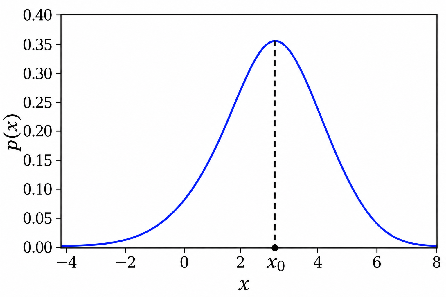
We find this point, which we’ll denote by $x_0$, using calculus:

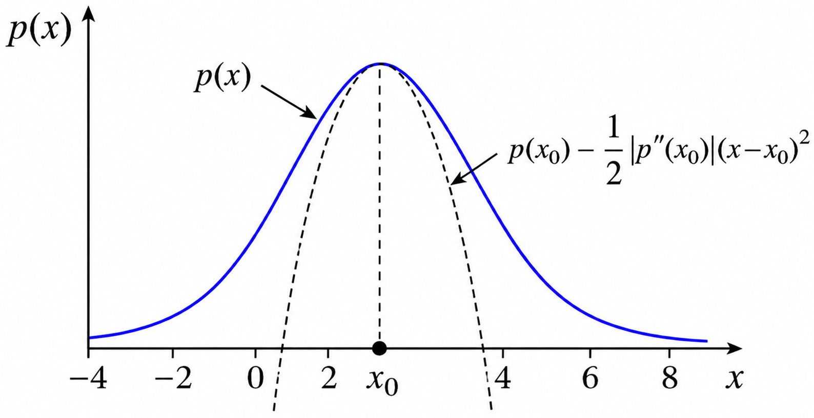
\[ \left.\frac{dp}{dx}\right|_{x=x_0} = 0 \quad \mbox{with} \quad \left.\frac{d^2p}{dx^2}\right|_{x=x_0} < 0 \ \text{(maximum)}. \]

To characterize the posterior $p(x)$, we look nearby. We want to know how sharp this maximum is: is $p(x)$ sharply peaked around $x=x_0$ or is the maximum kind-of shallow? To work this out we’ll do a Taylor expansion around $x=x_0$. The PDF $p(x)$ itself varies very rapidly, but since $p(x)$ is positive definite we can Taylor expand $\log p$ instead. (See the box below on “$p$ or $\log p$?” for a strict mathematical reason why it’s problematic for our purposes to directly Taylor expand $p(x)$ around its maximum.)

\[ \Longrightarrow\ L(x) \equiv \log p(x) = L(x_0) + \left.\frac{dL}{dx}\right|_{x = x_0}(x-x_0) + \frac{1}{2} \left.\frac{d^2L}{dx^2}\right|_{x = x_0}(x-x_0)^2 + \cdots \]

Note that $\left.\frac{dL}{dx}\right|_{x = x_0}=0$, because $L(x_0)$ is a maximum if $p(x_0)$ is, and $\left.\frac{d^2L}{dx^2}\right|_{x = x_0} < 0$. If we can neglect higher-order terms, then when we re-exponentiate,

\[ p(x) \approx A\, e^{\frac{1}{2}\left.\frac{d^2L}{dx^2}\right|_{x = x_0}(x-x_0)^2} , \]

with $A$ a normalization factor that originates in the $L(x_0)$ term. So in this general circumstance we get a Gaussian distribution. Comparing to

\[ p(x) = \frac{1}{\sqrt{2\pi\sigma^2}}e^{-(x-\mu)^2/\sigma^2} \quad\Longrightarrow\quad \mu = x_0, \ \sigma = \left(-\left.\frac{d^2L}{dx^2}\right|_{x=x_0}\right)^{-1/2}, \]

where we see the importance of the second derivative being negative.

We usually characterize the distribution by $x_0 \pm \sigma$ (e.g., with a point and symmetric error bars if this is data noise), because if it is a Gaussian this is sufficient to tell us the entire distribution. E.g., $n$ standard deviations is $n\times \sigma$. But for a Bayesian, the full posterior $p(x|D,I)$ for all $x$ is the general result, and $x = x_0 \pm \sigma$ may be only an approximate characterization.

To think about …

What if $p(x)$ is asymmetric? What if it is multimodal?

$p$ or $\log p$?

We motivated Gaussian approximations from a Taylor expansion to quadratic order of the logarithm of a PDF. What would go wrong if we directly expanded the PDF? Well, if we do that we get:

\[ p(x) \approx p(x_0) + \frac{1}{2}\left.\frac{d^2p}{dx^2}\right|_{x=x_0}(x-x_0)^2 \ \overset{x\pm\rightarrow\infty}{\longrightarrow} -\infty, \]

i.e., we get something that diverges as $x$ tends to either plus or minus infinity.

A PDF must be normalizable and positive definite, so this approximation violates these conditions!

The Central Limit Theorem#

Another reason a Gaussian PDF emerges in many situations is because the Central Limit Theorem (CLT) states that the sum of random variables drawn from all (or almost all) probability distributions will eventually produce Gaussians if the number of samples in each sum is large enough.

Central Limit Theorem

The sum of $n$ random values drawn from any PDF of finite variance $\sigma^2$ tends as $n \rightarrow \infty$ to be Gaussian distributed about the expectation value of the sum, with variance $n \sigma^2$.

Consequences:#

The mean of a large number of values becomes normally distributed regardless of the probability distribution the values are drawn from.
The binomial, Poisson, chi-squared, and Student’s t- distributions all approach Gaussian distributions in the limit of a large number of degrees of freedom (e.q., for large $n$ for binomial). This consequence is probably not immediately obvious to you from the statement of the CLT! (See the 📥 Demo: Visualization of the Central Limit Theorem notebook for an explanation of the Poisson distribution.)

Checkpoint Question

Why would we expect the CLT to work for a binomial distribution?

Hint

If we denote Bin($n,p$) as the binomial distribution for $n$ trials with probability $p$ of success, how is Bin($1,p$) related to Bin($n,p$)?

Answer

If we add up $n$ random variables from Bin($1,p$), each with value 0 or 1, this is equivalent to a Bin($n,p$) random variable with the same number of successes. So we already have a sum of random variables built in and the CLT will apply. (In more detail: getting $k$ ones and $n-k$ zeros from the $n$ Bin($1,p$) draws will have probability $p^k$ times $(1-p)^{n-k}$ times the number of combinations $n\choose k$. This is the same as the binomial probability for $k$ successes.)

CLT I: Moments of a PDF from a sum of random variables#

A Gaussian distribution is completely determined by its first and second moments (that is, its mean $\mu$ and variance $\sigma^2$). This is obvious if we know the distribution is a Gaussian, because its parametrization is fully specified given $\mu$ and $\sigma^2$. But this implies that all of the higher moments of a Gaussian distribution are fully determined by $\mu$ and $\sigma$. And if we find a distribution with the same pattern of higher moments, it must be a Gaussian. In this subsection we see how this observation leads us toward the CLT by returning to the analyses in Expectation values and moments.

It will be sufficient here (and much cleaner) to work with mean-zero distributions. The moments $\{m_k\}_{\mathcal{N}(0,\sigma^2)}$ of a mean-zero Gaussian distribution, which will be our target, can be found directly from the moment-generating function in (4.7):

\[ \{M_X(t)\}_{\mathcal{N}(0,\sigma^2)} = \exp(\frac{1}{2}\sigma^2 t^2) = \sum_{j=0}^{\infty} \frac{1}{j!}\left(\frac{\sigma^2 t^2}{2} \right)^j , \]

which means for $X \sim \mathcal{N}(0,\sigma^2)$ we find

(5.1)#\[\begin{split} \{m_k\}_{\mathcal{N}(0,\sigma^2)} = \mathbb{E}_{\mathcal{N}(0,\sigma^2)}[X^k] = \begin{cases} 0, & \text{if } k \text{ odd} \\ (2j-1)!! \sigma^{2j} & \text{if } k=2j \text{ even} \end{cases} = \begin{cases} 0, & \text{if } k \text{ odd} \\ \frac{k!}{2^{k/2} (k/2)!} \sigma^{k} & \text{if } k \text{ even} \end{cases} \ , \end{split}\]

where $(2j-1)!! = (2j-1)\cdot(2j-3)\cdots 3 \cdot 1$. Then all the odd moments are zero and $\{m_2\}_{\mathcal{N}(0,\sigma^2)}= \sigma^2$, $\{m_4\}_{\mathcal{N}(0,\sigma^2)} = 3\sigma^4$, $\{m_6\}_{\mathcal{N}(0,\sigma^2)} = 15\sigma^6$, and so on.

With those results in hand, we consider any distribution with mean zero and a finite variance $\sigma^2$. We consider a sum of $n$ random variables, all drawn independently from that same mean-zero (but not necessarily symmetric) distribution (hence they are iid), scaled by an overall $1/\sqrt{n}$ factor:

(5.2)#\[ X = \frac{1}{\sqrt{n}}(x_1 + x_2 + \cdots + x_n) = \sum_{j=1}^n \frac{x_j}{\sqrt{n}} . \]

Let’s consider moments $m_k = \mathbb{E}[X^k]$ of $X$ as $n$ gets large. $m_0 = 1$ and $m_1 = 0$, since the distribution is normalized and mean zero. By using the linearity of expectation values, the independence of the $x_i$, and $\mathbb{E}[x_i]=0$, we find $m_2$ directly:

\[ m_2 = \mathbb{E}[X^2] = \frac{1}{n} \left( n\cdot\mathbb{E}[x_1^2] + n (n-1)\cdot \mathbb{E}[x_1]\mathbb{E}[x_2]\right) = \sigma^2 . \]

We see that the scaling $1/\sqrt{n}$ in the definition of $X$ ensures an $n$-independent variance equal to the variance of the distribution. For $m_3$,

\[ \mathbb{E}[X^3] = \frac{1}{n^{3/2}} \left( n\cdot\mathbb{E}[x_1^3] + 0 \right) = \frac{1}{n^{1/2}}\mathbb{E}[x_1^3], \]

where the terms set equal to zero have at least one $\mathbb{E}[x_1] = 0$. Note that while the distribution can have a non-zero skewness (third moment), it will be suppressed as $n$ gets large. For $m_4$,

\[ \mathbb{E}[X^4] = \frac{1}{n^2}\left( n\cdot\mathbb{E}[x_1^4] + 3n(n-1)\cdot\mathbb{E}[x_1^2]\cdot\mathbb{E}[x_2^2] + 0 \right) = \frac{1}{n}\cdot\mathbb{E}[x_1^4] + 3(1-\frac{1}{n})\sigma^4 . \]

Now as $n$ gets large, $m_4$ reduces to the Gaussian kurtosis result of $3\sigma^4$. Note that as long as $n$ is finite, however, there will be non-Gaussian contributions (called excess kurtosis).

More generally, we see that the $\mathbb{E}[x_i^k]$ term in $m_k$ for $k\geq 2$ comes with a single factor of $n$, so it will always be suppressed by increasing powers of $\frac{1}{n}$. The only $n$-independent terms will be $k/2$ products of $\mathbb{E}[x_i^2] = \sigma^2$, with a coefficient that exactly matches $\{m_k\}_{\mathcal{N}(0,\sigma^2)}$.

Thus, the moments of the $X$ distribution will tend toward those of a Gaussian, meaning that the distribution itself tends towards a Gaussian distribution. That is the central limit theorem. Now let’s make a different construction towards the same end.

CLT II: Proof of the CLT#

Start with independent random variables $x_1,\cdots,x_n$ drawn from a distribution with mean $\langle x \rangle = 0$ and variance $\langle x^2\rangle = \sigma^2$, where

\[ \langle x^n \rangle \equiv \int x^n p(x)\, dx . \]

(Assuming mean zero is general, because we can always work with the distribution of $x - \mu$.) As in the last section, let

\[ X = \frac{1}{\sqrt{n}}(x_1 + x_2 + \cdots + x_n) = \sum_{j=1}^n \frac{x_j}{\sqrt{n}} , \]

scaling by $1/\sqrt{n}$ so that the variance of $X$ is constant in the $n\rightarrow\infty$ limit.

What is the distribution of $X$? $\Longrightarrow$ call it $p(X|I)$, where $I$ is the information about the probability distribution for $x_j$.

Plan: Use the sum and product rules and their consequences to relate $p(X)$ to what we know of $p(x_j)$. (Note: we’ll suppress $I$ to keep the formulas from getting too cluttered.)

\[\begin{split}\begin{align} p(X) &= \int_{-\infty}^{\infty} dx_1 \cdots dx_n\, p(X,x_1,\cdots,x_n) \\ &= \int_{-\infty}^{\infty} dx_1 \cdots dx_n\, p(X|x_1,\cdots,x_n)\,p(x_1,\cdots,x_n) \\ &= \int_{-\infty}^{\infty} dx_1 \cdots dx_n\, p(X|x_1,\cdots,x_n)\,p(x_1)\cdots p(x_n) . \end{align}\end{split}\]

State the rule used to justify each step

marginalization
product rule
independence

We might proceed by using a direct, normalized expression for $p(X|x_1,\cdots,x_n)$,

Checkpoint question

What is $p(X|x_1,\cdots,x_n)$?

Hint

If we know each of the $x_i$ values, we know $X$ exactly!

Answer

$p(X|x_1,\cdots,x_n) = \delta\Bigl(X - \frac{1}{\sqrt{n}}(x_1 + \cdots + x_n)\Bigr) = \frac{1}{2\pi} \int_{-\infty}^{\infty} d\omega \, e^{i\omega\Bigl(X - \frac{1}{\sqrt{n}}\sum_{j=1}^n x_j\Bigr)}$

and perform one of the integrations. Instead we will use a Fourier representation (see the answer to the Checkpoint question):

\[ p(X|x_1,\cdots,x_n) % = \delta\Bigl(X - \frac{1}{\sqrt{n}}(x_1 + \cdots + x_n)\Bigr) = \frac{1}{2\pi} \int_{-\infty}^{\infty} d\omega \, e^{i\omega\Bigl(X - \frac{1}{\sqrt{n}}\sum_{j=1}^n x_j\Bigr)} . \]

Substituting into $p(X)$ and gathering together all pieces with $x_j$ dependence while exchanging the order of integrations:

\[ p(X) = \frac{1}{2\pi} \int_{-\infty}^{\infty} d\omega \, e^{i\omega X} \prod_{j=1}^n \left[\int_{-\infty}^{\infty} dx_j\, e^{i\omega x_j / \sqrt{n}} p(x_j) \right] . \]

Observe that the terms in []s have factorized into a product of independent integrals and they are all the same (just different labels for the integration variables). Now we Taylor expand $e^{i\omega x_j/\sqrt{n}}$, arguing that the Fourier integral is dominated by small $x$ as $n\rightarrow\infty$. (When does this fail?) We find:

\[ e^{i\omega x/\sqrt{n}} = 1 + \frac{i\omega x}{\sqrt{n}} + \frac{(i\omega)^2 x^2}{2 n} + \mathcal{O}\left(\frac{\omega^3 x^3}{n^{3/2}}\right) . \]

Then, using that $p(x)$ is normalized (i.e., $\int_{-\infty}^{\infty} dx\, p(x) = 1$) and with the notation $\langle f(x) \rangle$ for the expectation value of $f(x)$,

\[\begin{split} \begin{align} \int_{-\infty}^{\infty} dx\, e^{i\omega x / \sqrt{n}} p(x)&= \int_{-\infty}^\infty dx\, p(x) \left[1 +\frac{ i \omega x}{\sqrt{n}} + \frac{(i \omega)^2 x^2}{2 n} + \ldots\right]\\ &=1 + \frac{i \omega}{\sqrt{n}} \langle x \rangle - \frac{\omega^2}{2 n} \langle x^2 \rangle + \langle x^3 \rangle \frac{\omega^3}{n^{3/2}}\\ &=1 - \frac{\omega^2 \sigma^2}{2 n} + \mathcal{O}\left(\frac{\omega^3}{n^{3/2}}\right) . \end{align} \end{split}\]

Now we can substitute into the posterior for $X$ and take the large $n$ limit:

\[\begin{split} \begin{align} p(X)&=\frac{1}{2 \pi} \int_{-\infty}^\infty d\omega\, e^{i \omega X} \left[1 - \frac{\omega^2 \sigma^2}{2 n} + \mathcal{O} \left(\frac{\omega^3}{n^{3/2}}\right)\right]^n\\ &\stackrel{n\rightarrow \infty}{\longrightarrow} \frac{1}{2 \pi} \int d\omega\, e^{i \omega X} e^{- \omega^2 \sigma^2/2}=\frac{1}{\sqrt{2 \pi}} e^{-X^2/(2 \sigma^2)}. \end{align} \end{split}\]

Checkpoint question

How did we use the large $n$ limit to get the first equality on the last line?

Answer

We used

\[ \lim_{n\rightarrow\infty} (1 + \frac{z}{n})^n = e^z \quad \text{for any $z$, here applied to } z = -\frac{\omega^2 \sigma^2}{2}. \]

We can understand this intuitively by multiplying out

\[\begin{split} \begin{align} \underbrace{(1 + \frac{z}{n})(1 + \frac{z}{n})\cdots(1 + \frac{z}{n})}_{n\ \text{terms}} &= 1 + n\cdot\frac{z}{n} + \binom{n}{2}\frac{z^2}{n^2} + \binom{n}{3}\frac{z^3}{n^3} + \ldots \\ &\overset{n\rightarrow\infty}{\longrightarrow} 1 + z + \frac{z^2}{2!} + \frac{z^3}{3!} + \ldots \end{align} \end{split}\]

In getting this result we have dropped terms that are of order $1/n$ and $1/n^2$. All terms that we dropped in truncating the Taylor expansions for each Fourier integral will also be suppressed by inverse powers (or half powers) of $n$.

Lead in to the demo notebook on visualizing the CLT#

Look at 📥 Demo: Visualization of the Central Limit Theorem for more intuitive insight into the CLT.

Things to think about:

What does “large” number of degrees of freedom actually mean? Does it matter where we look?
If we have a large number of draws from a uniform distribution, does the CLT imply that the histogrammed distribution should look like a Gaussian?
Can you identify a case (that we have seen) where the CLT will fail?

Answers

“Large” will depend on detail, but it is often surprising how few the number is before the CLT kicks in (e.g., often of order 30).
Yes! This is illustrated in the demo notebook.
The Cauchy distribution will fail because its variance is not finite.

More on Gaussian distributions

Contents

5.3. More on Gaussian distributions#

The near ubiquity of Gaussians#

The Gaussian is to statistics what the harmonic oscillator is to mechanics#

The Central Limit Theorem#

Consequences:#

CLT I: Moments of a PDF from a sum of random variables#

CLT II: Proof of the CLT#

Lead in to the demo notebook on visualizing the CLT#