40.4. Exercises

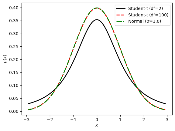
Exercise 40.1 (Scipy.stats)

Use scipy.stats to

• Find and print the mean and the variance;

• Find and print the 68% credible region (equal-tail interval);

• Draw and print 5 random samples;

• Plot the pdf (including at least 90% of the probability mass);

for

1. A student-t distribution with \(\nu=2\) degrees-of-freedom;

2. A student-t distribution with \(\nu=100\) degrees-of-freedom;

3. A standard normal distribution;

in all cases with the mode at 0.0.

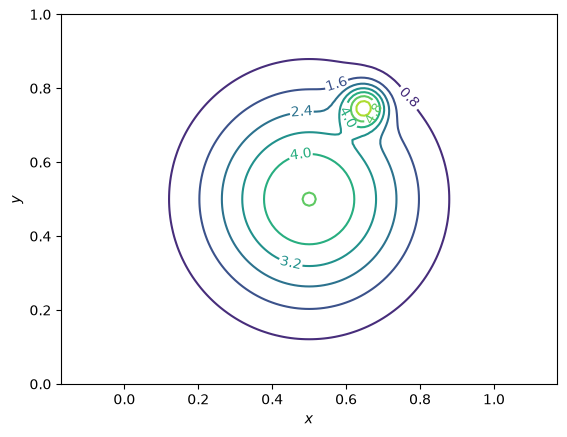
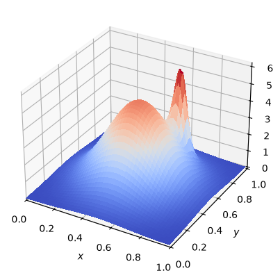
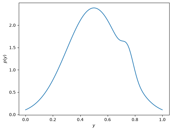
Exercise 40.2 (Bivariate pdf)

Consider the following (multimodal) bivariate pdf

\[ \p{x,y} = A_1 \exp\left(- \frac{(x-x_1)^2 + (y-y_1)^2}{2\sigma_1^2} \right) + A_2 \exp\left(- \frac{(x-x_2)^2 + (y-y_2)^2}{2\sigma_2^2} \right), \]

with \(A_1=4.82033\), \(x_1=0.5\), \(y_1=0.5\), \(\sigma_1=0.2\), and \(A_2=4.43181\), \(x_2=0.65\), \(y_2=0.75\), \(\sigma_2=0.04\).

Consider the domain \(x,y \in [0,1]\) and use relevant python modules / methods to

• Plot contour levels of this pdf (useful methods: np.meshgrid and plt.contour);

• Make a three-dimensional plot of the pdf (useful methods: plt.subplots(subplot_kw={"projection": "3d"}) and plt.plot_surface);

• Compute and plot the marginal pdf \(\p{y}\) (useful method: scipy.integrate.quad)

Solutions

Solution to Exercise 40.1 (Scipy.stats)

See the code example in the hidden code block below.

Show code cell content

Hide code cell content

import scipy.stats as stats
import matplotlib.pyplot as plt
import numpy as np
fig, ax = plt.subplots(1, 1)

# Define a student-t distribution with location=0.0 and scale = 1.0
# and \nu=2 degreefs of freedom 
df=2
my_student_t_rv = stats.t(df, loc=0.0, scale=1.0)

# An appropriate mesh for plotting
x = np.linspace(my_student_t_rv.ppf(0.05),my_student_t_rv.ppf(0.95), 100)

print(f'=========\n Student-t distribution df={df}\n=========')
# Extract and print the mean and variance
print(f'The mean is {my_student_t_rv.mean():3.1f}')
print(f'The variance is {my_student_t_rv.var():3.1f}')

# The 68% credible interval (approximately one sigma)
(min68,max68) = my_student_t_rv.interval(0.68)
print(f'The 68% credible interval is [{min68:4.2f},{max68:4.2f}]')

# Draw random samples.
print(my_student_t_rv.rvs(size=5))
# Plot
ax.plot(x, my_student_t_rv.pdf(x), 'k-', lw=2, label=f'Student-t (df={df})')

# Define a student-t distribution with location=0.0 and scale = 1.0
# and \nu=100 degreefs of freedom 
df=100
my_student_t_rv = stats.t(df, loc=0.0, scale=1.0)

print(f'=========\n Student-t distribution df={df}\n=========')
# Extract and print the mean and variance
print(f'The mean is {my_student_t_rv.mean():3.1f}')
print(f'The variance is {my_student_t_rv.var():3.1f}')

# The 68% credible interval (approximately one sigma)
(min68,max68) = my_student_t_rv.interval(0.68)
print(f'The 68% credible interval is [{min68:4.2f},{max68:4.2f}]')

# Draw random samples.
print(my_student_t_rv.rvs(size=5))
# Plot
ax.plot(x, my_student_t_rv.pdf(x), 'r--', lw=2, label=f'Student-t (df={df})')

# Define a normal distribution with location=0.0 and scale = 1.0
scale = 1.0
my_normal_rv = stats.norm(loc=0.0, scale=scale)

print(f'=========\n Normal distribution (sigma = {scale:3.1f})\n=========')
# Extract and print the mean and variance
print(f'The mean is {my_normal_rv.mean():3.1f}')
print(f'The variance is {my_normal_rv.var():3.1f}')

# The 68% credible interval (approximately one sigma)
(min68,max68) = my_normal_rv.interval(0.68)
print(f'The 68% credible interval is [{min68:4.2f},{max68:4.2f}]')

# Draw random samples.
print(my_normal_rv.rvs(size=5))
# Plot
ax.plot(x, my_normal_rv.pdf(x), 'g-.', lw=2, label=fr'Normal ($\sigma$={scale})')
ax.legend(loc='best')
ax.set_xlabel(r'$x$')
ax.set_ylabel(r'$p(x)$');

=========
 Student-t distribution df=2
=========
The mean is 0.0
The variance is inf
The 68% credible interval is [-1.31,1.31]
[-2.22452528 -5.48129769  0.10656564  3.95149027 -0.40276024]
=========
 Student-t distribution df=100
=========
The mean is 0.0
The variance is 1.0
The 68% credible interval is [-1.00,1.00]
[ 0.05424355 -0.35627293  0.47390846 -0.05151771  0.68070388]
=========
 Normal distribution (sigma = 1.0)
=========
The mean is 0.0
The variance is 1.0
The 68% credible interval is [-0.99,0.99]
[-0.29848653 -0.68745332  1.65497762 -1.26022769 -2.27193524]

Solution to Exercise 40.2 (Bivariate pdf)

See the code example in the hidden code block below.

Show code cell content

Hide code cell content

import numpy as np
import matplotlib.pyplot as plt
from matplotlib import cm

def pdf(x,y,A1=4.82033,x1=0.5,y1=0.5,sigma1=0.2,\
            A2=4.43181,x2=0.65,y2=0.75,sigma2=0.04):
	return A1*np.exp(-((x-x1)**2 + (y-y1)**2)/(2*sigma1**2)) + \
		A2*np.exp(-((x-x2)**2 + (y-y2)**2)/(2*sigma2**2))

delta = 0.01
x = np.arange(0.0, 1.0, delta)
y = np.arange(0.0, 1.0, delta)
X, Y = np.meshgrid(x, y)
p = pdf(X,Y)

fig, ax = plt.subplots(1, 1)
CS = ax.contour(X, Y, p)
ax.axis('equal')
ax.set_xlim(0.0,1.0)
ax.set_xlabel(r'$x$')
ax.set_ylim(0.0,1.0)
ax.set_ylabel(r'$y$')
ax.clabel(CS, inline=True, fontsize=10)

fig3d, ax3d = plt.subplots(subplot_kw={"projection": "3d"})
# Plot the surface.
surf = ax3d.plot_surface(X, Y, p, cmap=cm.coolwarm,
                       linewidth=0, antialiased=False)
ax3d.set_xlim(0.0,1.0)
ax3d.set_xlabel(r'$x$')
ax3d.set_ylim(0.0,1.0)
ax3d.set_ylabel(r'$y$')
ax3d.set_zlabel(r'$p(x,y)$');

import scipy.integrate as integrate
y = np.linspace(0,1,100)
pdfy=np.zeros_like(y)
for iy,yi in enumerate(y):
	I = integrate.quad(pdf, 0, 1, args=(yi))
	pdfy[iy] = I[0]
fig_pdfy, axy = plt.subplots(1, 1)
axy.plot(y,pdfy)
axy.set_xlabel(r'$y$')
axy.set_ylabel(r'$p(y)$');

Ignoring fixed x limits to fulfill fixed data aspect with adjustable data limits.