32.2. Neural networks in the large-width limit#
The big picture is that the neural network acts like a parameterized function
where the input vector is \(x\) (we don’t use boldface or arrows for this vector) and \(\pars\) is the collective vector of all the parameters (weights and biases). In order to understand this we need a framework and an approximation scheme. Effective (field) theory and large-width limit of the network is a compelling path.
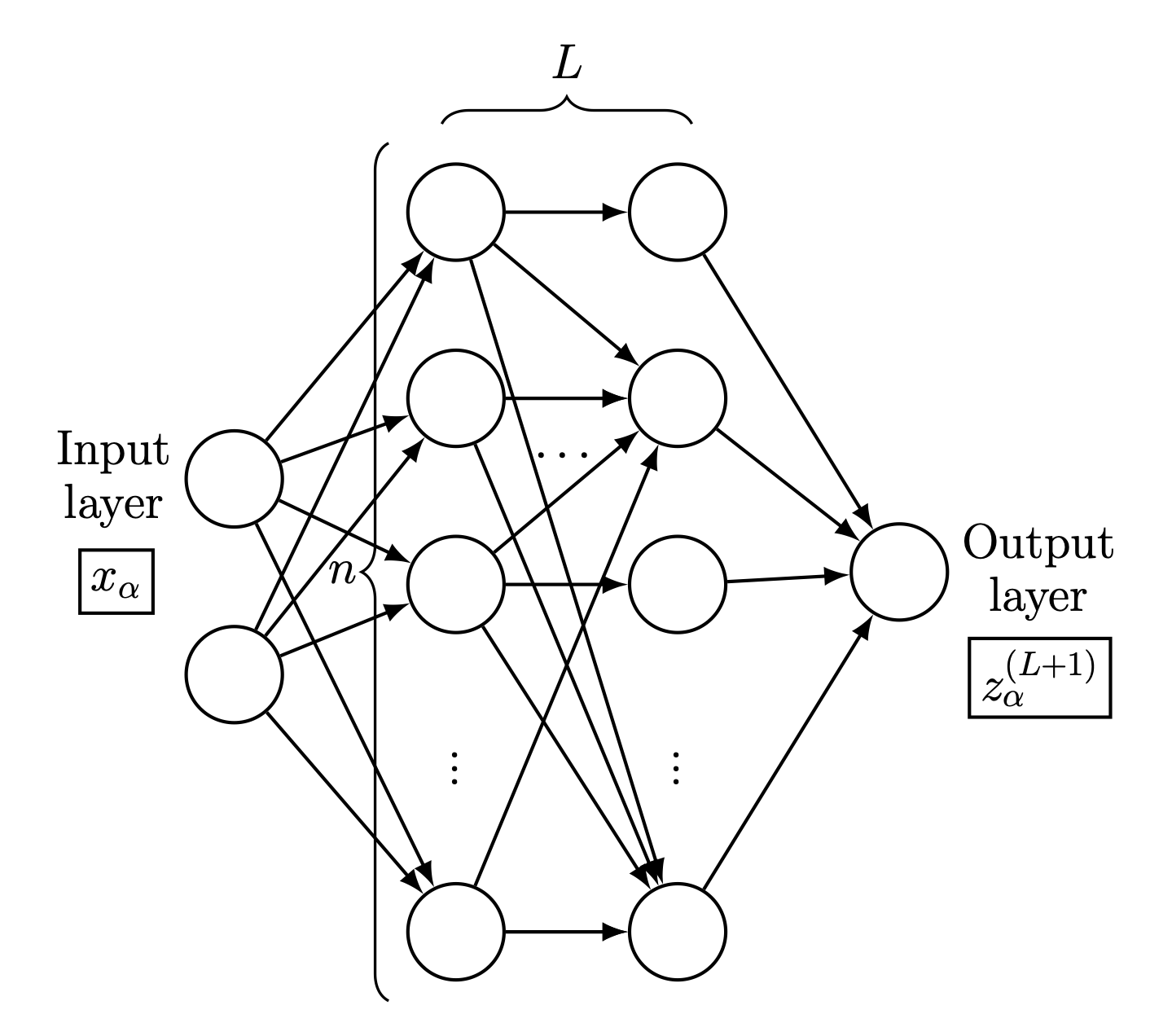
Fig. 32.1 Schematic of a feed-forward neural network with two inputs \(x_{\alpha}\) and one output \(z_{\alpha}^{(L+1)}\), where \(\alpha\) is an index running over the dataset \(\mathcal{D}\). The width is \(n\) and the depth is \(L+1\), with \(L\) being the number of hidden layers. The neurons are totally connected (some lines are omitted here for clarity). For the examples shown in this chapter, the inputs are the number of protons \(Z\) and neutrons \(N\) and the output is the mass (or, equivalently, the binding energy) of the corresponding nuclide (see Fig. 32.2).#
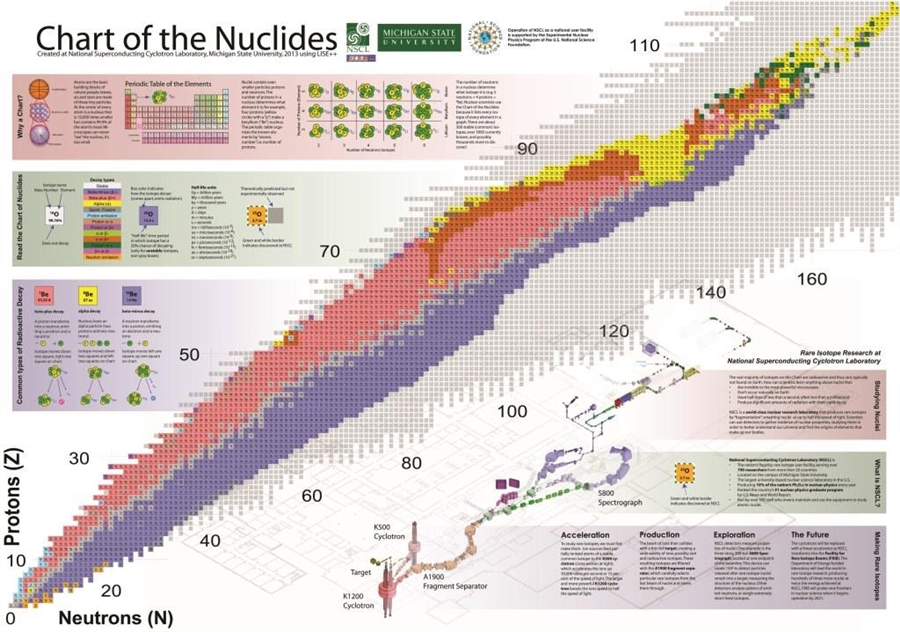
Fig. 32.2 Chart of the nuclides.#
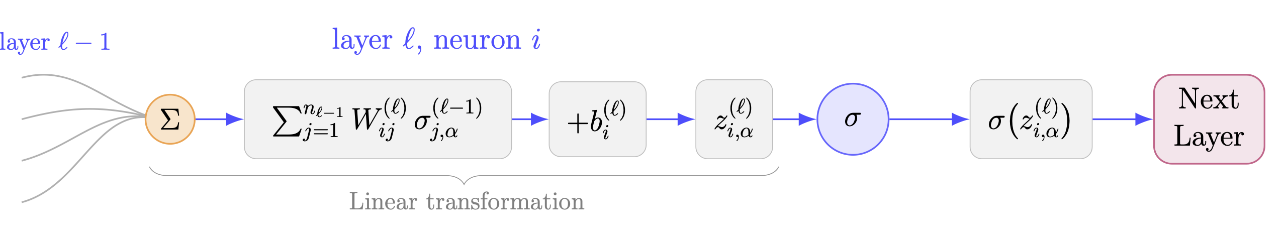
Fig. 32.3 Schematic of a neuron within a neural network. In the layer \(\ell\), the product between the weight matrix \(W^{(\ell)}\) and the previous layers’ output \(\sigma^{(\ell-1)}\) is summed over the width of the prior layer \(n_{\ell-1}\), and a bias vector \(b^{(\ell)}\) is added, forming the preactivation \(z^{(\ell)}\). The activation function \(\sigma\) acts on the preactivation to yield the output \(\sigma \bigl(z^{(\ell)}\bigr)\) (also notated \(\sigma^{(\ell)}\)) to be passed to the next layer.#
For a given initialization of the network parameters \(\pars\), the preactivations and the output function \(f\) are uniquely determined. However, a repeated random initialization of \(\pars\) induces a probability distribution on preactivations and \(f\). Explicit expressions for these probability distributions in the limit of large width \(n\) can be derived, with the ratio of depth to width revealed as an expansion parameter for the distribution’s action. The output distribution in a given layer \(\ell\) refers to the distribution of preactivations \(z^{(\ell)}_{j,\alpha}\). This choice allows for parallel treatment of all other layers with the function distribution in the output layer.
To achieve the desired functional relationship between \(x_{i,\alpha}\) and \(y_{j,\alpha}\), a neural network is trained by adjusting the weights and biases in each layer according to the gradients of the loss function \(\mathcal{L}\bigl(f(x,\pars),y\bigr)\). The loss function quantifies the difference between the network output \(f(x,\pars)\) and the output data \(y\), and the goal of training is to minimize \(\mathcal{L}\bigl(f(x,\pars),y\bigr)\). The gradients of \(\mathcal{L}\bigl(f(x,\pars),y\bigr)\) with respect to the network parameters \(\pars\) depend on the size of the output, as well as the architecture hyperparameters. It is known empirically that poor choices of architecture and/or initialization lead to exploding/vanishing gradients in the absence of adaptive learning algorithms, and this was problematic for training networks for many years.
The ANN output function \(f(x,\pars)\) for any fixed \(\pars\) (that is, specified weights and biases) is a deterministic function. But, as already stressed, with repeated initializations of the ANN with \(\pars\) drawn from random distributions, the network acquires a probability distribution over functions \(p\left(f(x)|\mathcal{D}\right)\). Again, \(\mathcal{D}\) is used to represent the data set of inputs and outputs that the network is finding a relationship between. In the pre-training case, this quantity simply refers to the inputs \(x_\alpha\) for the network.
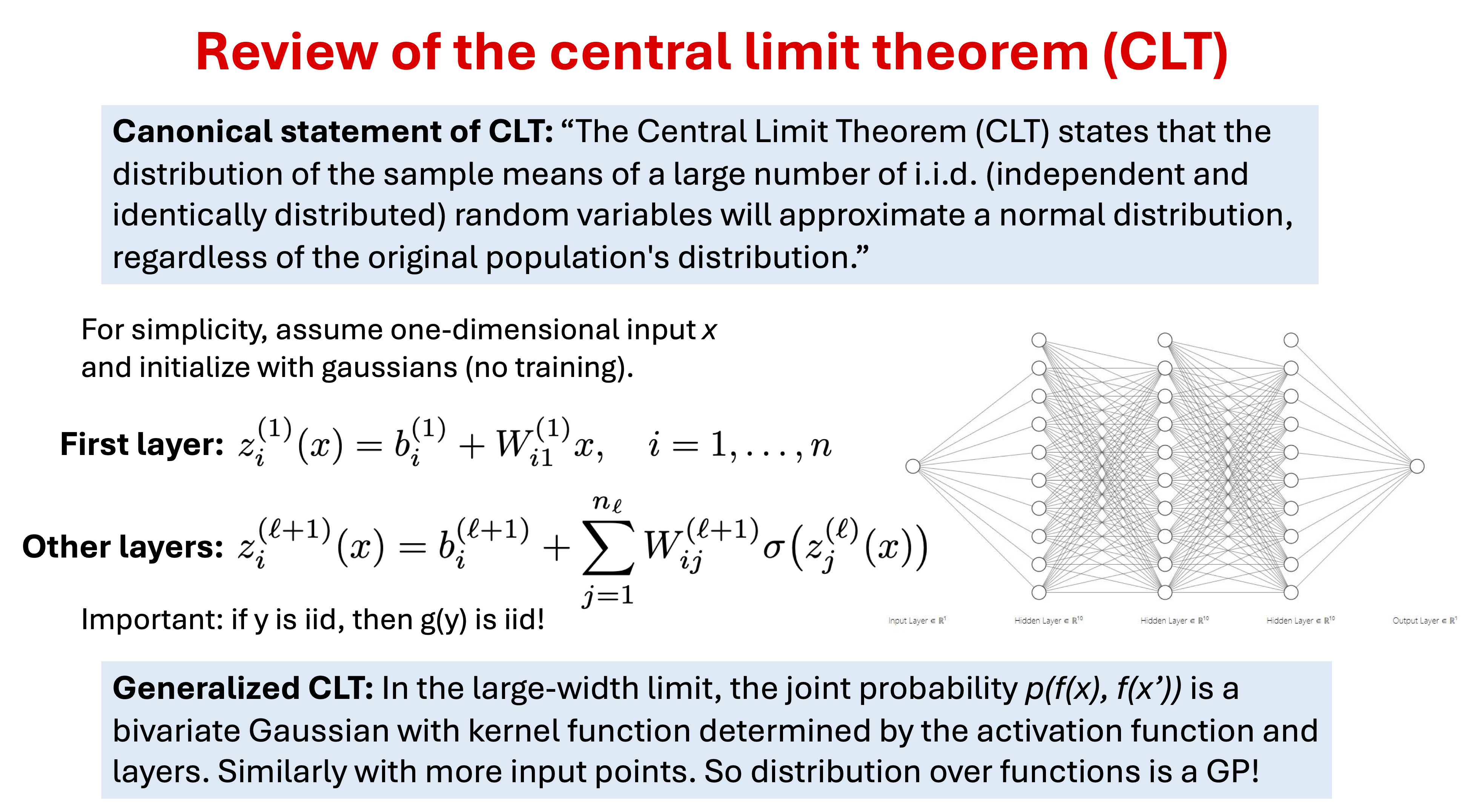
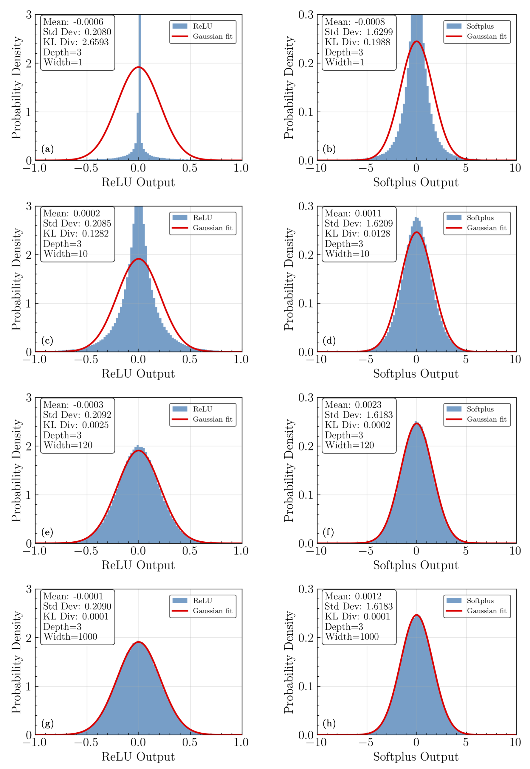
Fig. 32.4 Final layer ANN output distributions from repeated sampling at the same input point, each plot being a different width. There are two hidden layers. ReLU activation is on the left; Softplus activaiton is on the right. The widths vary from 1 up to 1000 neurons per layer.#
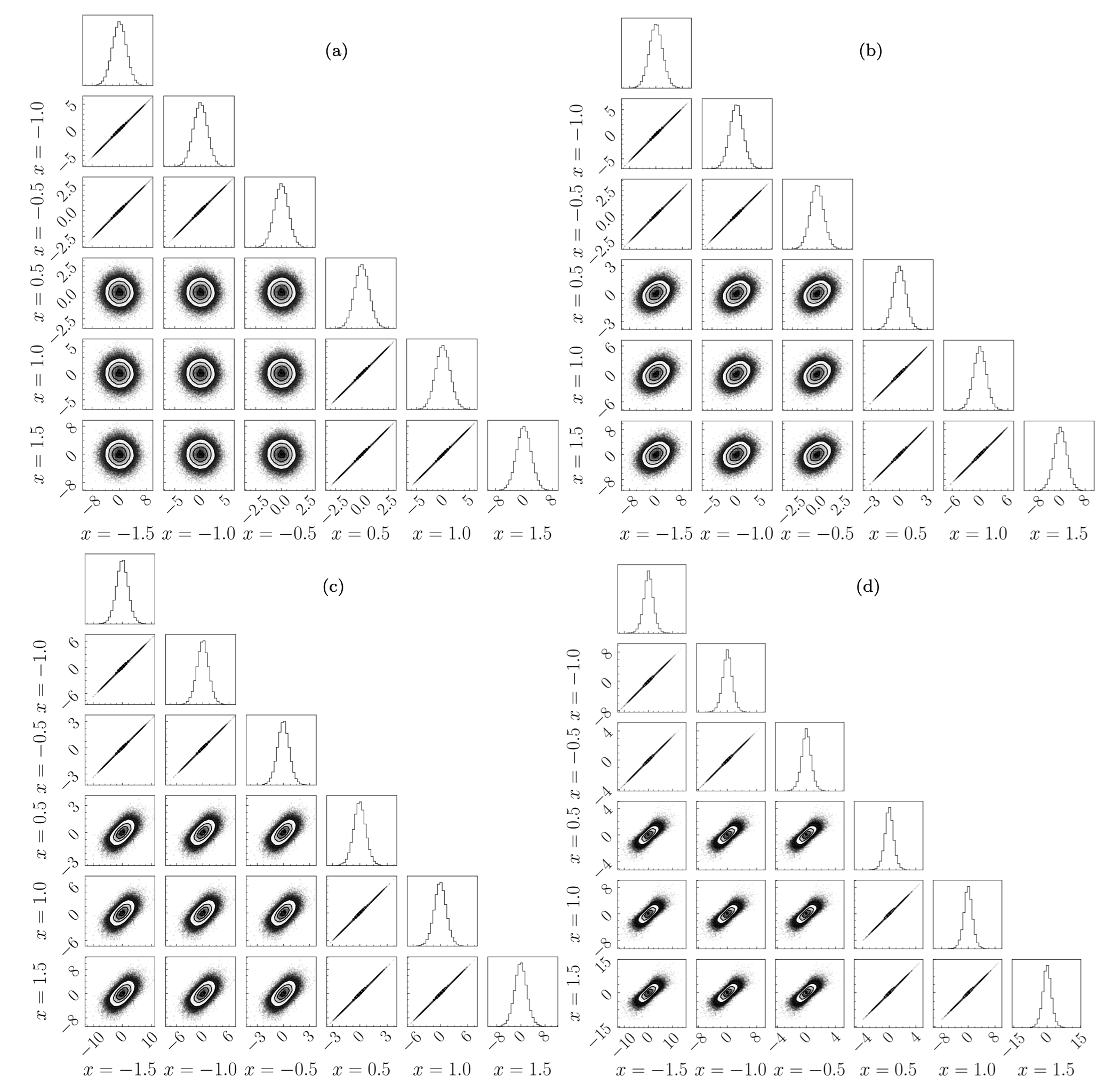
Fig. 32.5 Corner plots for ReLU activation function outputs. The corner plots all feature ReLU networks of a fixed width of 120 neurons, and depths of (a) 1, (b) 2, © 4, and (d) 8. The addition of hidden layers introduces correlations to the network output distributions.#
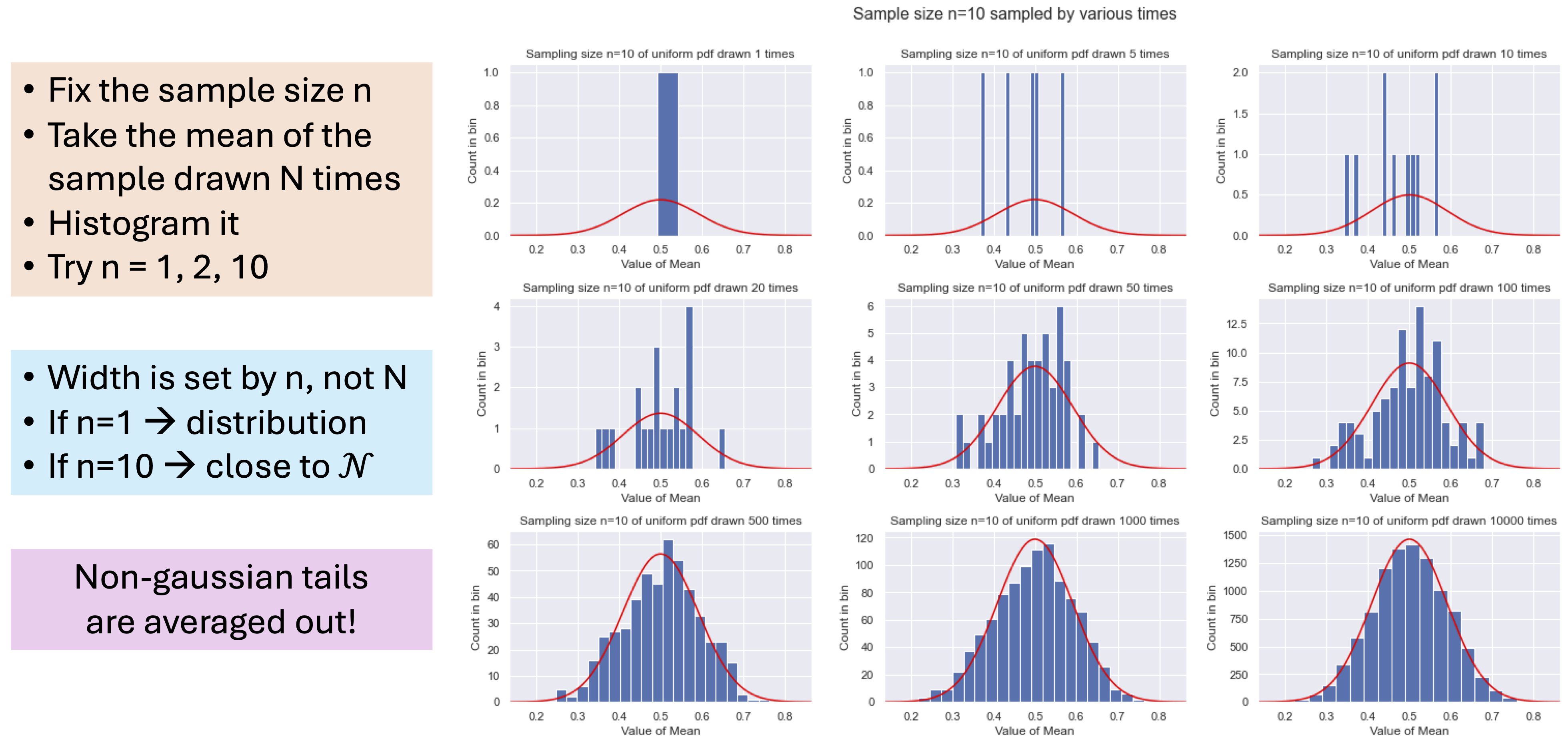
Fig. 32.6 Intuition for the central limit theorem (CLT).#
Summary: What is the prior distribution \(p(f(x;θ)|I)\)?#
The network’s weights and biases \(\thetavec\) are initialized as independent and identically distributed random variables (zero mean, we can take as Gaussian).
Neural network of given architecture induces a probability distribution of preactivations \(z\) at a given layer \(\ell\).
The preactivation of final (output) layer is \(f(x)\).
The Central Limit Theorem kicks in as the width \(n\) goes to infinity, so these distributions should become (correlated) Gaussians, i.e., Gaussian processes.
Claim: if we back off from this limit, neural networks can be studied using perturbation theory, with an expansion parameter: depth/width.
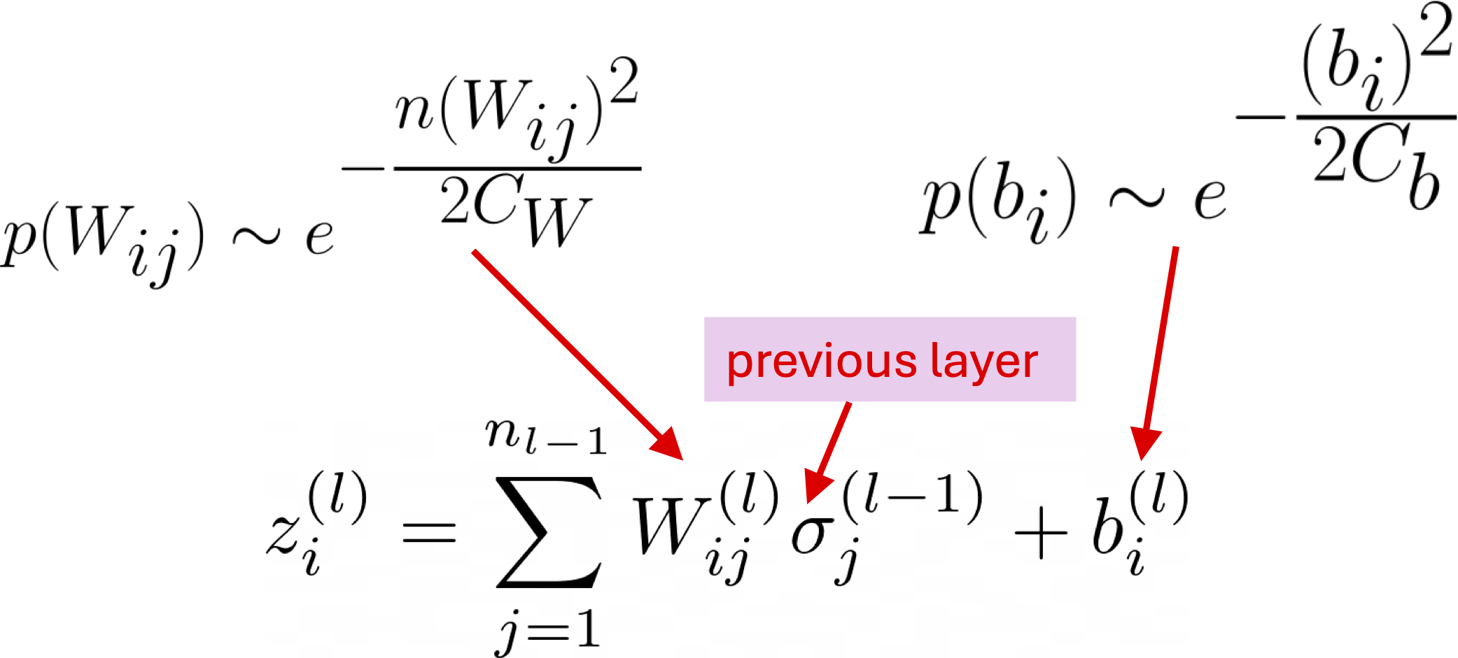
Fig. 32.7 Initialization distributions#