34.4. Demo: RBM vs. HO expansion vs. GP

Setting up an example

As an explicit illustrative example we consider a simple anharmonic oscillator in quantum mechanics with potential:

\[ V(r; {{\pars}}) = V_{\text{HO}}(r) + \sum_{n=1}^3 {\para_n} e^{-r^2/\sigma_n^2} \quad\mbox{ with } \sigma_n = [0.5, 2, 4] \; \mathrm{fm} \]

Checkpoint question

How do you know that this potential is affine in the sense of (34.7)?

Answer

The dependence on \(\pars = \{\para_1,\para_2,\para_3\)} is factored from the \(r\) and \(\sigma_n\) dependence. That is, the potential is the sum of terms, each of which is independent of \(\pars\) or the product of a function of some \(\para_i\) (in this case a linear function) times a function independent of \(\pars\).:::

Checkpoint question

Would the potential be affine if we chose to vary the \(\sigma_n\) parameters?

Answer

No, because the \(\sigma_n\) appear nonlinearly with the \(r\) dependence; they cannot be factored out.:::

In this example, the high fidelity solution is from the numerical solution of the time-independent Schrodinger equation with a fine mesh in coordinate space.

Training and testing the emulator

Following the MOR paradigm, we take snapshots of the high-fidelity wave function at various training parameters \(\{\pars_i\}\) and collect them into our basis \(X\). Matrix elements in the reduced space (a \(n_b \times n_b\) matrix) are

\[ \mel{\psi(\pars_i)}{V(r;\pars)} {\psi(\pars_j} = \mel{\psi(\pars_i)}{V_{\text{HO}}(r)} {\psi(\pars_j)} + \sum_{n=1}^3 \pars_n \mel{\psi(\pars_i)}{e^{-r^2/\sigma_n^2}}{\psi(\pars_j)} , \]

which is manifestly affine. Thus the matrix elements on the right side can be calculated in advance (offline stage) once the snapshots training parameters are chosen.

Here, we choose \(n_b = 6\) training points randomly and uniformly distributed in the range \([-5, 5]\),MeV for all \(\para_n\); 50 validation parameter sets are chosen within the same range. For illustration, we take three of the validation parameter sets we sampled and compare the exact and emulated wave functions for both the RBM and HO emulators in Fig. 34.6 and Fig. 34.7. Although both the reduced basis and HO basis are rich enough to capture the main effects of varying \(\pars\), the RBM emulator is much more effective at capturing the fine details of the wave function.

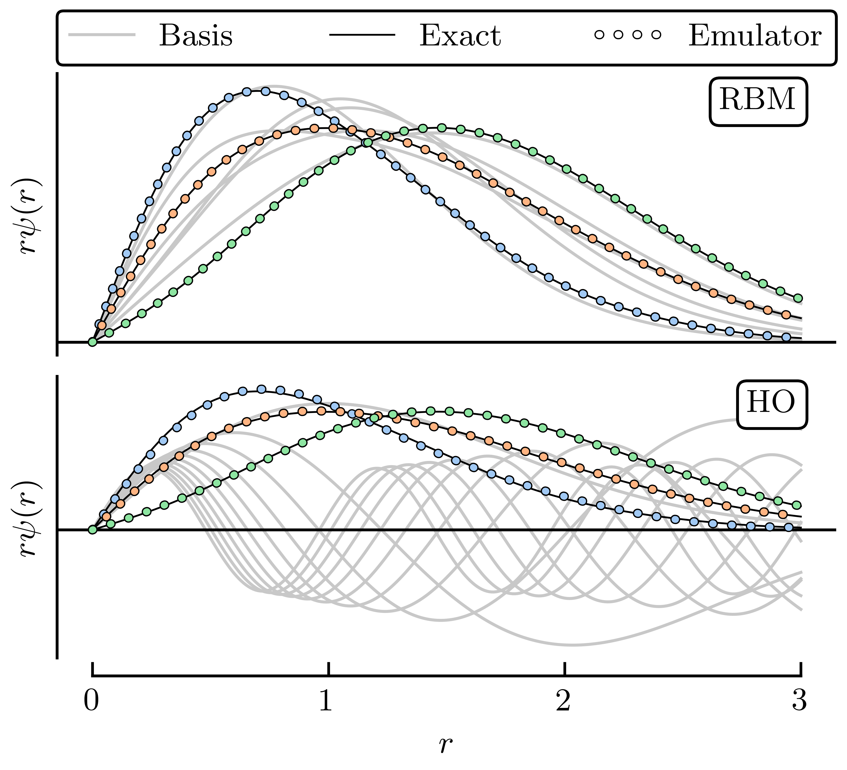
Fig. 34.6 Comparison of RBM and HO snapshot wave functions for the illustrative toy example.

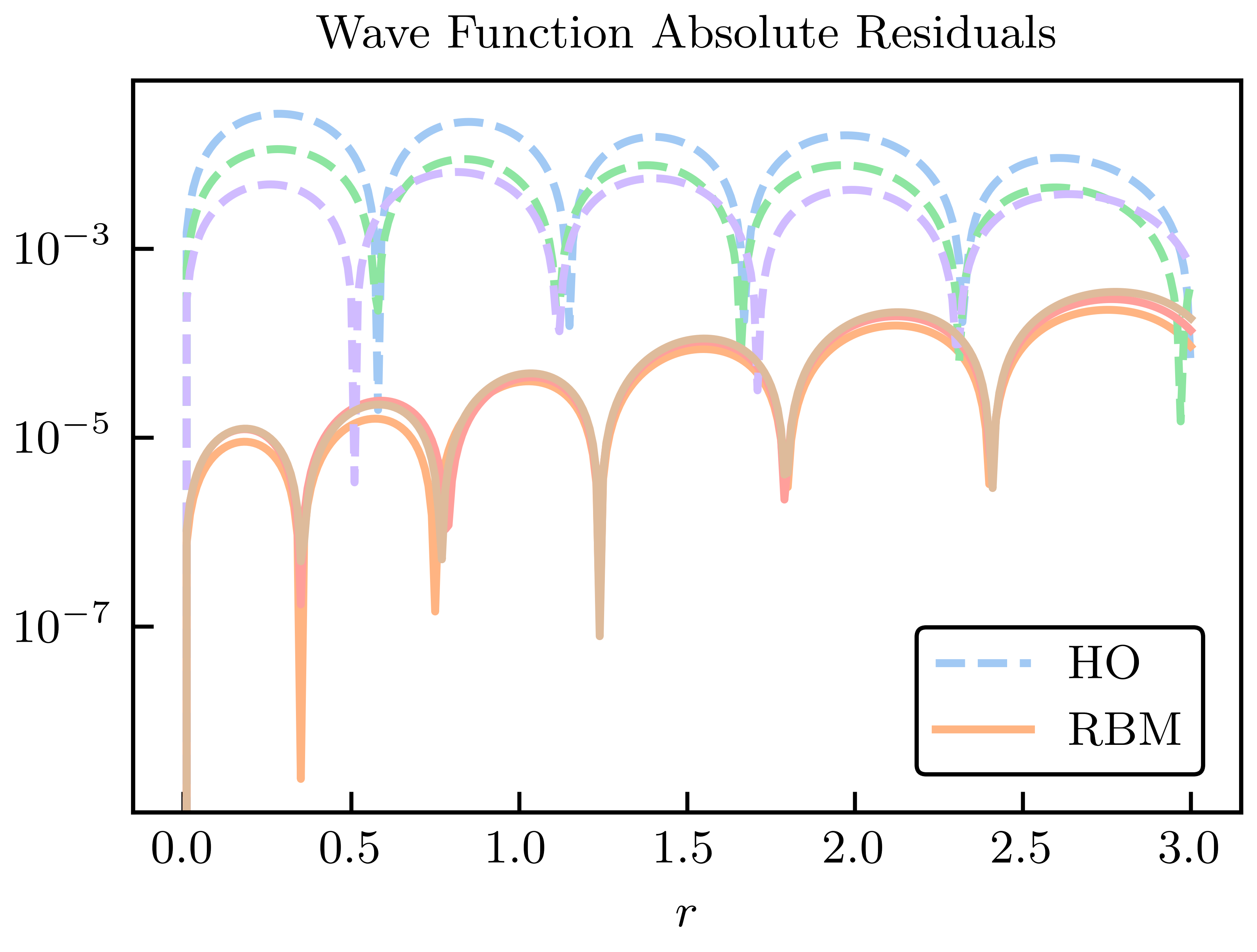
Fig. 34.7 Absolute residuals compared to the high-fidelity solution for the HO and RBM emulators.

We can add a comparison to a Gaussian process emulator. GPs are non-parametric, non-intrusive machine learning models for both regression and classification tasks. Their popularity stems partly from their convenient analytical form and flexibility in effectively modeling various types of functions. GPs benefit from treating the underlying set of codes as a black box, but this is a double-edged sword.

A Gaussian process (GP) emulator is constructed from a set of training points, with uncertainties, by conventional GP regression formulas. This provides interpolated values with error bands. No information about the model is needed, so this is a data-driven emulator. In this example we use two independent GPs to emulate the ground-state energy and the corresponding radius expectation value. Each GP uses a Gaussian covariance kernel and is fit to the observable values at the same values of \(\pars_i\) used to train the RBM emulator. We use the maximum likelihood values for the hyperparameters.

Because the GP relaxes to the prior mean on distances of order the correlation length, the extrapolation performance of GP emulators is poor unless there are constraints built into the GP kernel. Comparisons to RBM emulators for realistic nuclear physics problems are shown in Fig. 34.2 and Fig. 34.3.

Comparing results for observables

For our demonstration example, the absolute residuals for the energy and radius at the validation points for each of the RBM, HO, and GP emulators are shown in Fig. 34.8 and Fig. 34.9.

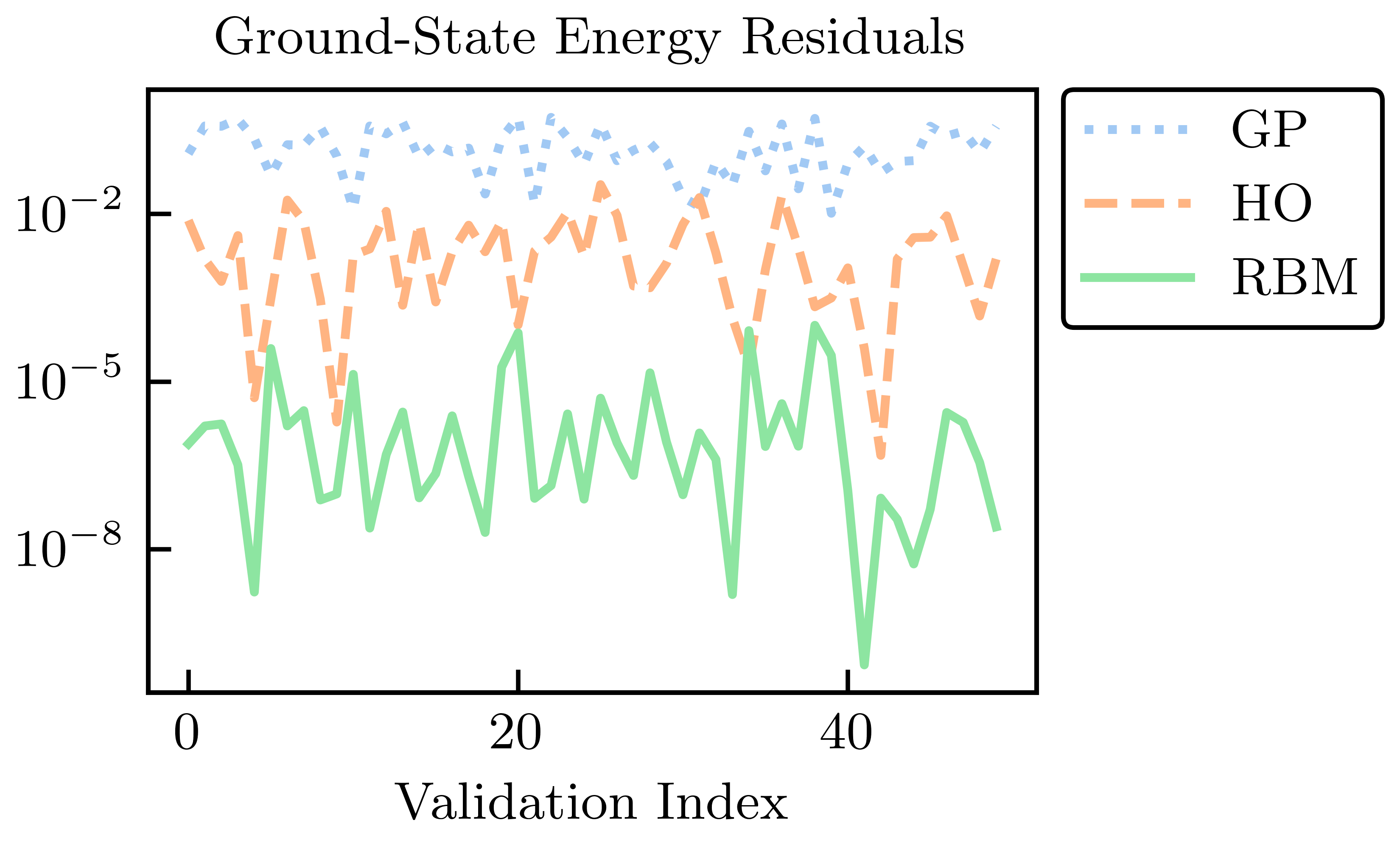
Fig. 34.8 Energy residuals across a test set for EC and GP emulation, compared with an ordinary variational calculation with the six lowest harmonic oscillator wave functions (no anharmonic piece)

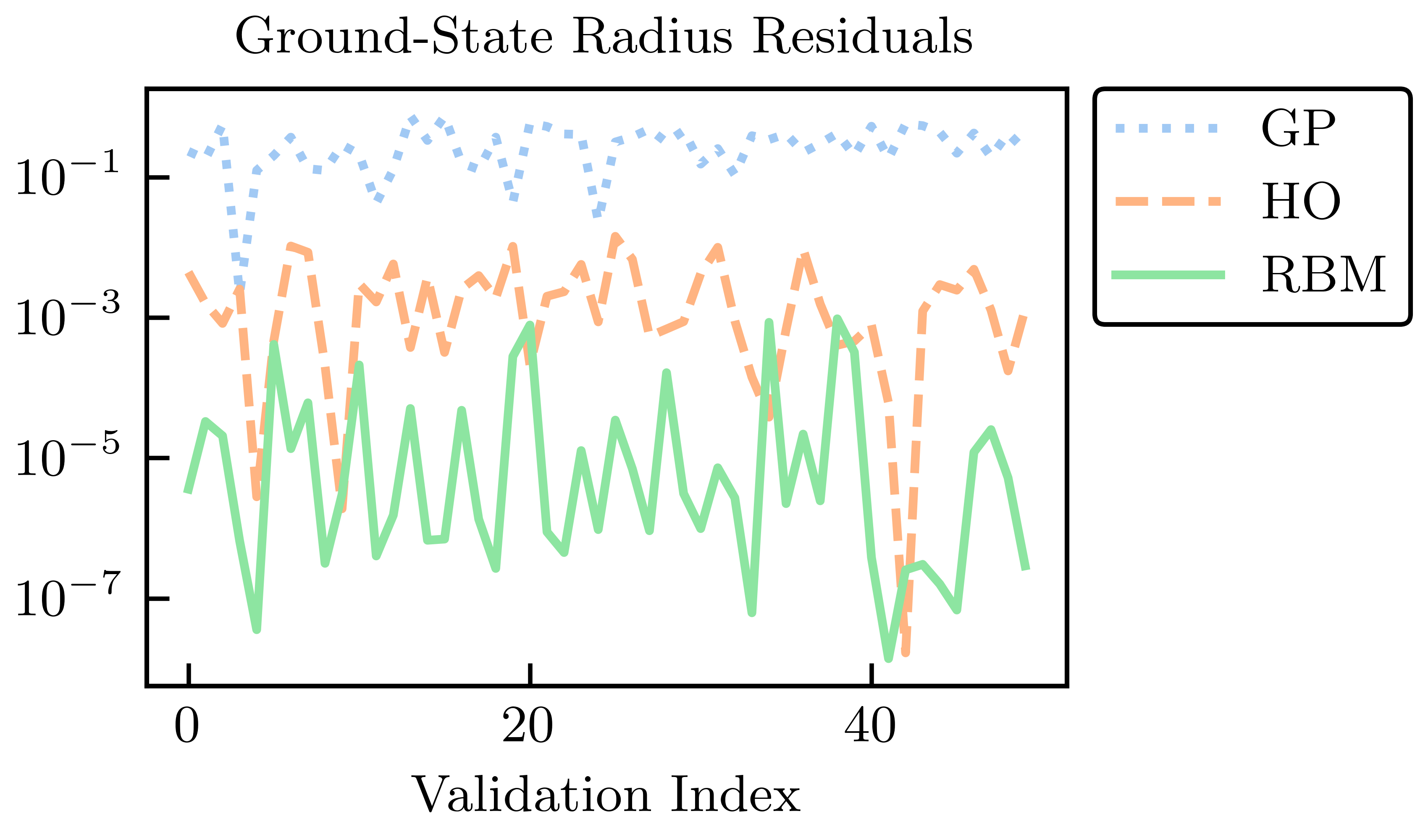
Fig. 34.9 Radius residuals across a test set for EC and GP emulation, compared with an ordinary variational calculation with the six lowest harmonic oscillator wave functions (no anharmonic piece)

We see that the GP emulators perform the worst, despite being trained on the values of the energies and radii themselves to perform this emulation task. Furthermore, the GP emulator’s ability to extrapolate beyond the support of its training data is often poor unless great care is taken in the design of its kernel and mean function. The GP suffers from what, in other contexts, could be considered its strength: because it treats the high-fidelity system as a black box (although some information can be conveyed via physics-informed priors for the hyperparameters), it cannot use the structure of the high-fidelity system to its advantage. Note that the point here is not that it is impossible to find some GP that can be competitive with other RBM emulators after using expert judgment and careful (i.e., physics-informed) hyperparameter tuning. Rather, we emphasize that with the reduced-order models, remarkably high accuracy is achieved without the need for such expertise.

The HO emulator performs better than the GP emulator, but it was not “trained” per se, it was merely given a basis of the lowest six HO wave functions as a trial basis, from which a reduced-order model was derived. However, the HO emulator can still outperform the GP emulator because it takes advantage of the structure of the high-fidelity system: it is aware that the problem to be solved is an eigenvalue problem, for this is built into the emulator itself. This feature permits a single HO emulator to emulate the wave function, energy, and radius simultaneously.

The RBM emulator’s performance is the best, which typically demonstrates higher accuracies than the HO and GP emulators by multiple orders of magnitude. The RBM emulator combines the best ideas from the other emulators. Like the GP, the RBM emulator uses evaluations of the eigenvalue problem as training data. However, its “training data” are curves (i.e., the wave functions) rather than scalars (e.g., eigen-energies), like the GP is trained upon. Like the HO emulator, the RBM emulator takes advantage of the structure of the system when projecting the high-fidelity system to create the reduced-order model. With these strengths, the RBM emulator is highly effective in emulating bound-state systems, even with only a few snapshots and far from the support of the snapshots.

The summary here is that the GP does not use the structure of the high-fidelity system to its advantage; the HO emulator knows the problem to be solved is an eigenvalue problem but nothing more; the RBM (aka EC) training data are curves rather than scalars, taking advantage of system structure.