11.3. Maximum Entropy for reconstructing a function from its moments

Here we use Maximum Entropy to reconstruct some simple functions from their moments, using the formulation by Mead and Papanicolaou, J. Math. Phys. 24, 2404 (1984). The context is answering the question: If we know some (or all) of the moments of a one-dimensional distribution \(p(x)\), how can we find the PDF? This question was asked in Section 4.4 and we repeat the definitions from there. We define the moments \(m_k\) for integer \(k\) as

\[ m_k = \int_S x^k\, p(x)\, dx, \qquad k= 0,1,2,\ldots, \]

where \(S\) denotes the support of the PDF (e.g., \((-\infty,\infty)\) for a Gaussian or \([0,1]\) for a Beta distribution). So \(m_0 = 1\), the mean \(\mu\) is \(m_1\), the variance \(\sigma^2\) is \(m_2 - m_1^2\), and so on.

If we have only a finite number \(N+1\) of moments, this is an underdetermined inverse problem. We solve it by maximizing the entropy associated with \(p(x)\) subject to the condition that the first \(N+1\) moments be equal to the true moments \(m_k\), \(k=0,1,\ldots,N\). To carry this out we introduce \(N+1\) Lagrange multipliers \(\lambda_k\) and maximize the functional \(S = S[p]\) defined by

\[ S = -\int_a^b [p(x)\ln p(x) - p(x)] dx + \sum_{k=0}^{N} \lambda_k \Bigl(\int_a^b x^k p(x) dx - m_k \Bigr). \]

We take the functional derivative with respect to \(p(x)\) and set it equal to zero, yielding

\[ \frac{\delta S}{\delta{p(x)}} = 0 \ \Longrightarrow \ p(x) = p_N(x) = \exp\Bigl(-\lambda_0 - \sum_{k=1}^N \lambda_k x^k \Bigr), \]

which will be our expression when we know the \(\lambda_k\)s. We have \(N+1\) nonlinear equations for those \(N+1\) unknown after taking partial derivatives with respect to the \(\lambda_k\)s and setting them to zero, yielding

\[ \int_a^b x^k p_N(x) dx = m_k, \quad k=0,1,\ldots,N. \]

We will assume that \(p(x)\) is normalized, i.e., that \(m_0 = 1\). This implies that the \(k=0\) equation can be used to solve for \(\lambda_0\), which defines the partition function (and a Boltzmann factor as the integrand):

\[ e^{\lambda_0} = \int_a^b dx\, \exp\Bigl(- \sum_{k=1}^N \lambda_k x^k \Bigr) \equiv Z. \]

We perform a Legendre transformation to go from the free energy \(\ln Z\) to the effective potential \(\Gamma = \Gamma(\lambda_1, \lambda_2,\ldots,\lambda_N)\)

\[ \Gamma = \ln Z + \sum_{k=1}^N m_k\lambda_k . \]

Given initial guesses for the \(\lambda\)s, we will simply numerically minimize \(\Gamma\) to find the \(\lambda\)s and then evaluate \(p_N(x)\).

Benchmark case

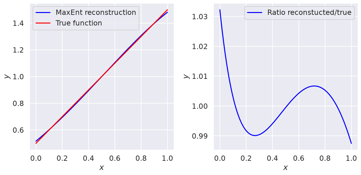
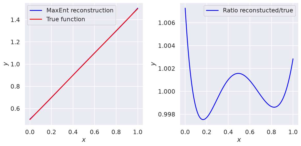
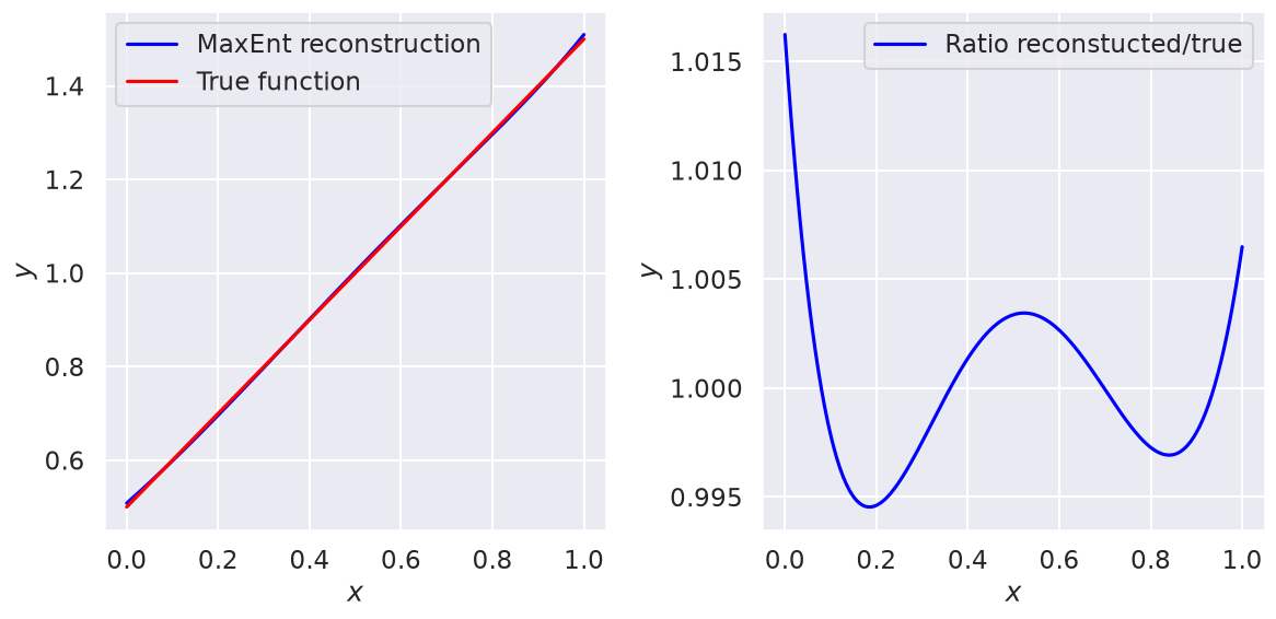
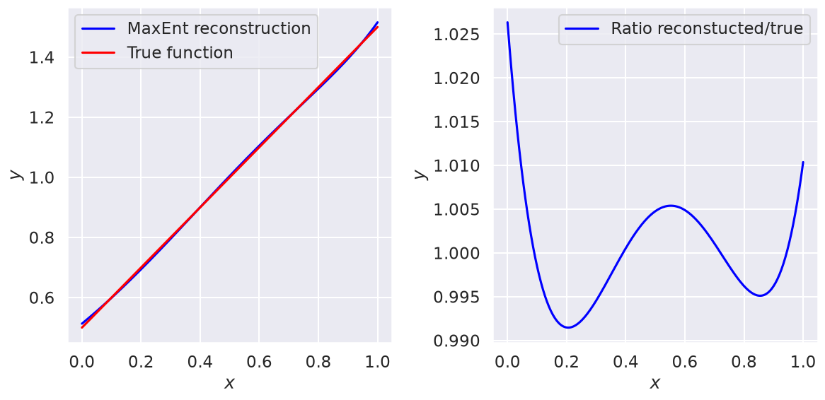
As a benchmark, we consider the (normalized) distribution \(p(x)=x + 1/2\) in the domain \(0 \leq x \leq 1\). For \(N=2\) to \(N=5\), we minimize the effective potential, starting from \(\lambda_k = 1\) for all \(k\), and then reconstruct and plot the result, comparing to the exact result.

Show code cell source

Hide code cell source

%matplotlib inline
import numpy as np

import scipy.stats as stats
from scipy.stats import norm, uniform

from scipy.optimize import minimize

import scipy.integrate as integrate

import matplotlib.pyplot as plt

import ipywidgets as widgets
from ipywidgets import HBox, VBox, Layout, Tab, Label, Checkbox, Button
from ipywidgets import FloatSlider, IntSlider, Play, Dropdown, HTMLMath 

from IPython.display import display

import seaborn as sns; sns.set(); sns.set_context("talk")

def Boltzmann(x, lambdas):
    """
    Defines the "Boltzmann factor".  The Lagrange multiplier array lambdas
    can be any size. 
    """
    return np.exp( -np.sum( [ lambdas[i] * x**(i+1) 
                              for i in range(len(lambdas)) ] 
                          ) 
                 )

def Z(lambdas):
    """
    Defines the partition function.
    Note shift in index because of way Python subscripts arrays.
    Using quad from scipy.integrate.
    """
    return integrate.quad(Boltzmann, 0., 1., args=lambdas, epsrel=1.e-16)[0]

def EffectivePotential(lambdas, mus):
    """
    Defines the effective potential.
    lambdas and mus must be numpy arrays.
    """
    return np.log( Z(lambdas) ) + mus @ lambdas 

def Px(x_pts, lambdas):
    """
    MaxEnt estimate for polynomial P(x).  
    Takes a numpy array x_pts and the vector lambdas as input.
    """
    norm = integrate.quad(Boltzmann, 0., 1., lambdas, 
                          epsrel=1.e-14)[0]
    return [Boltzmann(x, lambdas) / norm for x in x_pts]

def y_true(x_pts):
    """Simple test function: y = x + 1/2"""
    return 0.5 + x_pts

def lambdas_min(mus):
    """Minimize the effective potential with respects to the lambdas,
       given an array of mu values (mus).
       We need to specify a small tolerance (tol) to ensure the output
       from minimize is sufficiently precise.
       At high orders this seems to have trouble converging to the best
       minimum.  Sensitive to where one starts and the method.
    """
    lambdas0 = 1.0 * np.ones(len(mus))  # start the minimization with all ones
    res = minimize(EffectivePotential, lambdas0, args=mus)
    return np.array(res.x)

def plot_lines(mus):
    x_pts = np.linspace(0, 1, 301)   # mesh for plots (enough so smooth)
    y_reconstruct = Px(x_pts, lambdas_min(mus))

    font_size = 18
    plt.rcParams.update({'font.size': font_size})
    
    fig = plt.figure(figsize=(12,6))

    ax = fig.add_subplot(1,2,1)
    ax.plot(x_pts, y_reconstruct, label="MaxEnt reconstruction", color="blue")
    ax.plot(x_pts, y_true(x_pts), label="True function", color="red")
    ax.set_xlabel(r'$x$')
    ax.set_ylabel(r'$y$')
    ax.legend()

    ax2 = fig.add_subplot(1,2,2)
#     ax2.plot(x_pts, y_true(x_pts) - y_reconstruct, 
#             label="residual", color="blue")
    ax2.plot(x_pts, y_reconstruct / y_true(x_pts), 
            label="Ratio reconstucted/true", color="blue")
    ax2.set_xlabel(r'$x$')
    ax2.set_ylabel(r'$y$')
    ax2.legend()

    fig.tight_layout()    

N=2 moments

Show code cell source

Hide code cell source

mus2=np.array([7/12, 5/12])
plot_lines(mus2)
print('Moments: ', mus2)
print('Minimized Lagrange multipliers lambdas: ',lambdas_min(mus2))

Moments:  [0.58333333 0.41666667]
Minimized Lagrange multipliers lambdas:  [-1.5892963   0.53499597]

N=3 moments

Show code cell source

Hide code cell source

mus3=np.array([7/12, 5/12, 13/40])
plot_lines(mus3)
print('Moments: ', mus3)
print('Minimized Lagrange multipliers lambdas: ',lambdas_min(mus3))

Moments:  [0.58333333 0.41666667 0.325     ]
Minimized Lagrange multipliers lambdas:  [-1.84589891  1.13219435 -0.38049834]

N=4 moments

Show code cell source

Hide code cell source

mus4=np.array([7/12, 5/12, 13/40, 4/15])
plot_lines(mus4)
print('Moments: ', mus4)
print('Minimized Lagrange multipliers lambdas: ',lambdas_min(mus4))

Moments:  [0.58333333 0.41666667 0.325      0.26666667]
Minimized Lagrange multipliers lambdas:  [-1.69942478  0.54755159  0.45576187 -0.39286306]

N=5 moments

Show code cell source

Hide code cell source

mus5=np.array([7/12, 5/12, 13/40, 4/15, 19/84])
plot_lines(mus5)
print('Moments: ', mus5)
print('Minimized Lagrange multipliers lambdas: ',lambdas_min(mus5))

Moments:  [0.58333333 0.41666667 0.325      0.26666667 0.22619048]
Minimized Lagrange multipliers lambdas:  [-1.57582227  0.23066907  0.48946635  0.13622942 -0.36347669]

Checkpoint question

Does the result improve from \(N=2\) to \(N=3\)? From \(N=3\) to \(N=4\)? From \(N=4\) to \(N=5\)?

Answer

There is clear improvement from \(N=2\) to \(N=3\), but not beyond that. Note that at N=4 the minimum found is: -0.04278640499674846, but there is also: -0.04279159257882259. How could you persuade Python to find this slightly better minimum? Does it help?

Exercises

Exercise 11.1

Copy the code defined here (open Show code cell source) to a Jupyter notebook (or write your own version) to produce a MaxEnt reconstruction of \(y(x)=2x\) for \(0 \leq x \leq 1\).

Exercise 11.2

MaxEnt doesn’t even care about essential singularities. Compute the moments for \(y(x)=1/\mu_0 \exp(-1/x)\) and reconstruct it. Note that you need to choose the constant \(\mu_0\) so that \(y\) can be interpreted as a probability distribution (i.e., normalized). [Copy the code defined here (open Show code cell source) to a Jupyter notebook (or write your own version)].

Exercise 11.3

MaxEnt does care about some things, though. Repeat the last exercise but for \(P(x)=4x-1\) and see what happens. Can you figure out why MaxEnt failed for this function?