31.4. Demo: Gaussian processes#
Gaussian processes as high-dimensional Gaussian distributions#
A Gaussian process (GP) is a collection of random variables, \(( Y_x )_{x\geq 0}\) (labeled by a continuous index \(x\)) such that any finite number of such variables has a joint, multivariate Gaussian distribution. In fact, this implies that the GP is a continuous-time stochastic process although we use \(x\) instead of \(t\) as our index variable.
We will typically consider any number \(n=1, 2, \ldots\) of indices with \(0 \leq x_1 < x_2, < \ldots < x_n\).
For any \(n\), the GP is completely determined by its mean vector \(\boldsymbol{\mu}\), with \(\mu_i = \mathbb{E}(Y_i)\), and covariance matrix \(\boldsymbol{\Sigma}\), with \(\Sigma_{ij} = \text{Cov}(Y_i,Y_j)\), for \(i,j \in 1, \ldots, n\) and \(Y_k \equiv Y(x_k)\).
Although a GP can formally involve any valid covariance matrix, we will restrict ourselves to positive covariances \(\Sigma_{ij}>0\). Furthermore, we will usually have correlations that become weaker with increasing distance in the index variable, i.e.,
(recall that \(\rho_{ij} = \frac{\Sigma_{ij}}{\sigma_i \sigma_j}\), where \(\sigma_i^2 = \Sigma_{ii})\).
Multivariate normal distributions#
Consider the set of random variables
These have a multivariate normal (Gaussian) distribution if the linear combination
has a univariate normal distribution for all real numbers \((a_1, a_2, \ldots, a_k)\). The multivariate normal distribution is completely specified by the mean vector \(\boldsymbol{\mu}\) and the covariance matrix \(\boldsymbol{\Sigma}\). In fact, the random variable \(Z \sim \mathcal{N}(\mu_Z,\sigma_Z^2)\) with
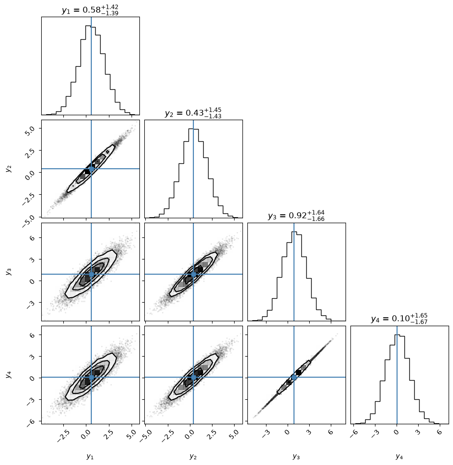
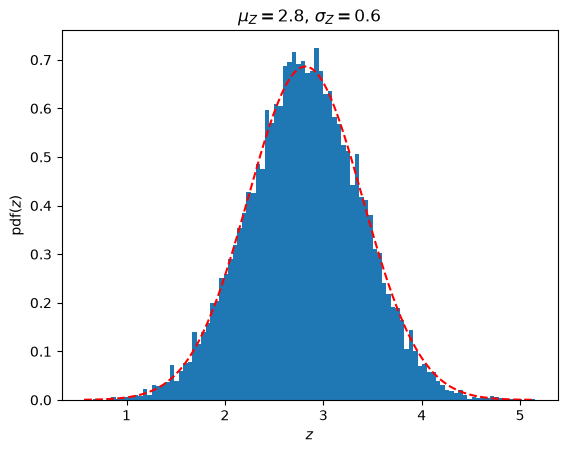
Make a corner plot with samples from bi- and univariate marginals. Note that corner shows a histogram and iso-probability contours in the densest region (and samples outside). Then plot the histogram of samples together with the analytical distribution.
Sampling and plotting multivariate Gaussians#
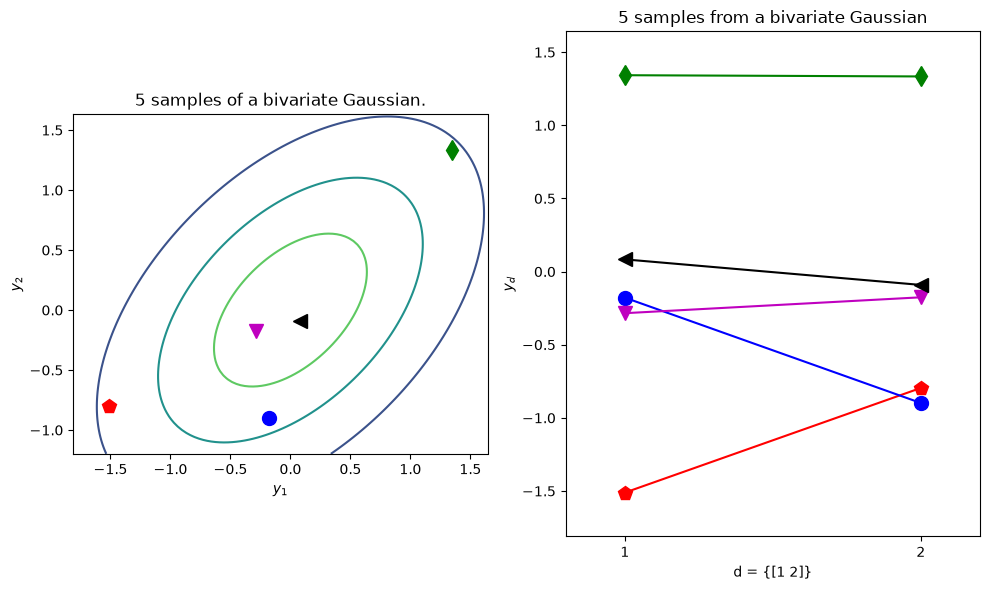
Test two different ways of plotting a bivariate Gaussian.
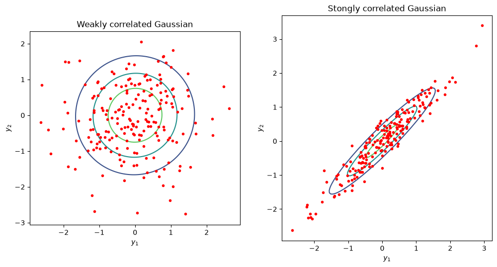
Repeat as before, but now we’ll plot many samples from two kinds of Gaussians: one which with strongly correlated dimensions and one with weak correlations
But let’s plot them as before dimension-wise…
Which one is which?
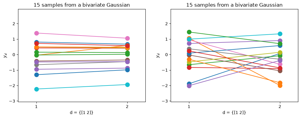
The strongly correlated Gaussian gives more “horizontal” lines in the dimension-wise plot.
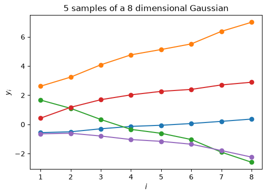
More importantly, by using the dimension-wise plot, we are able to plot Gaussians which have more than two dimensions. Below we plot N samples from a D=8-dimensional Gaussian.
Because I don’t want to write down the full 8x8 covariance matrix, I define a “random” one through a mathematical procedure that is guaranteed to give me back a positive definite and symmetric matrix (i.e. a valid covariance). More on this later.
Covariance matrix:
[[2.02 2.09 2.12 2.15 2.16 2.17 2.19 2.21]
 [2.09 2.45 2.69 2.89 2.98 3.07 3.27 3.42]
 [2.12 2.69 3.1  3.48 3.66 3.83 4.23 4.55]
 [2.15 2.89 3.48 4.05 4.33 4.59 5.22 5.73]
 [2.16 2.98 3.66 4.33 4.65 4.96 5.72 6.33]
 [2.17 3.07 3.83 4.59 4.96 5.32 6.19 6.9 ]
 [2.19 3.27 4.23 5.22 5.72 6.19 7.38 8.35]
 [2.21 3.42 4.55 5.73 6.33 6.9  8.35 9.54]]
Eigenvalues all larger than zero
[35.57+0.j  2.75+0.j  0.19+0.j  0.  +0.j  0.  +0.j  0.  +0.j  0.  +0.j
  0.  -0.j]
Taking this even further, we can plot samples from a 200-dimensional Gaussian in the dimension-wise plot.
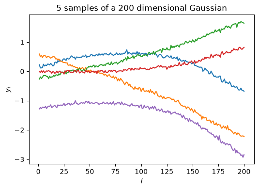
We see that each sample now starts looking like a “smooth” curve (notice that the random variables are highly correlated). This illustrates why a GP can be seen as an infinite dimensional multivariate Gaussian that can be used as a prior over functions.
Mean and covariance function#
Similarly to how a D-dimensional Gaussian is parameterized by its mean vector and its covariance matrix, a GP is parameterized by a mean function and a covariance function. These can be written as functions of the index variable \(x\). We’ll assume (without loss of generality) that the mean function is \(\mu(x) = \mathbf{0}\). As for the covariance function, \(C(x,x')\), it is a function that receives as input two locations \(x,x'\) belonging to the input domain, i.e. \(x,x' \in \mathcal{X}\), and returns the value of their co-variance.
In this way, if we have a finite set of input locations we can evaluate the covariance function at every pair of locations and obtain a covariance matrix \(\mathbf{C}\). We write:
Covariance functions, aka kernels#
We saw above their role for creating covariance matrices from training inputs, thereby allowing us to work with a finite domain when it is potentially infinite.
We’ll see below that the covariance function is what encodes our assumption about the GP. By selecting a covariance function, we are making implicit assumptions about the shape of the function we wish to encode with the GP, for example how smooth it is.
Even if the covariance function has a parametric form, combined with the GP it gives us a nonparametric model. In other words, the covariance function is specifying the general properties of the GP function we wish to encode, and not a specific parametric form for it.
Below we define two very common covariance functions: The RBF (also known as Exponentiated Quadratic or Gaussian kernel) which is differentiable infinitely many times (hence, very smooth),
where \(Q\) denotes the dimensionality of the input space. Its parameters are: the lengthscale, \(\ell\) and the signal variance \(\sigma_f^2\). We also note that this kernel is stationary, meaning that it only depends on the distance \(\left| \mathbf{x}_{i} - \mathbf{x}_{j} \right|\).
There are many other kinds of kernels. An example of a non-stationary one is the linear kernel:
Below, we will implement and investigate them.
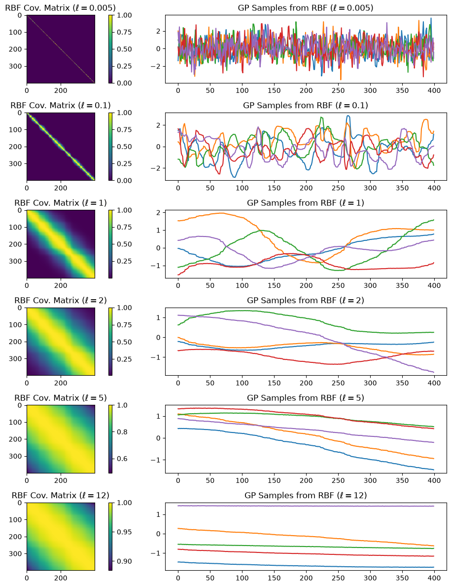
The RBF kernel (a.k.a Gaussian)#
Given hyperparameters \(\boldsymbol{\alpha}\), we plot the resulting covariance matrix and samples from a GP with this covariance function.
Example: GP models for regression#
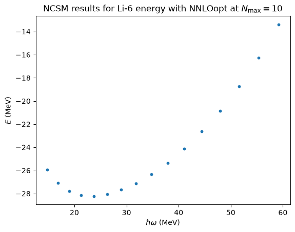
No-core shell model \(\hbar\omega\) dependence#
Import some NCSM data from Phys. Rev. C 97, 034328 (2018).
Test our GP by training on every third data point and validate on the rest.
k1 : 2.24**2
k1__constant_value : 5.0
k1__constant_value_bounds : (1e-05, 100000.0)
k2 : RBF(length_scale=10)
k2__length_scale : 10.0
k2__length_scale_bounds : (1e-05, 100000.0)
       l = 15.329
 sigma_f = 1.384
sigma_nu = 1e-06
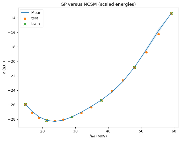
Print the largest ratios (predict-true)/predict for the validation data.
Validation result: Ratio true/predict in [0.9930,1.0303]