34.3. RBM emulators#
Eigenvector continuation#
Synopsis#
In this chapter we consider emulation based on reduced basis models (RBM) as introduced under the name eigenvector continuation (EC). This method is very useful for applications where the computer model can be phrased as an eigenvalue problem. For example, consider the prediction of the eigenenergy of a quantum state such that \(M(\pars) = E(\pars)\) is obtained by solving the Schrödinger equation
This equation can be projected onto a suitable basis and thereby expressed as a matrix eigenvalue problem for which the eigenstate, \(| \psi(\pars) \rangle\), becomes an eigenvector. In certain applications it might be that the dimension \(N\) of this basis is very large. In quantum many-body simulations you might have \(N \sim 10^9\) or even larger.
For a statistical analysis we must explore the consequences of varying the numerical values of \(\pars\). In, e.g., MCMC sampling we might need many thousands (or much more) model evaluations and must therefore seek a way to mitigate the computational cost of solving for \(E_\odot \equiv E(\pars_\odot)\) (and \(| \psi_\odot \rangle \equiv | \psi(\pars_\odot) \rangle\)) for any target parametrization \(\pars_\odot\) of interest.
The key insight of eigenvector continuation [FHI+18] is that although an eigenvector resides in a linear space with enormous dimensions, the eigenvector trajectory generated by smooth changes of the Hamiltonian matrix is well approximated by a very low-dimensional manifold in many applications.
We therefore start by constructing a basis of \(n \ll N\) eigenvectors \(\{ | \psi_i \rangle \}_{i=1}^n\) obtained from exact solutions of the Schrödinger equation at different model parametrizations \(\{ \pars_i \}_{i=1}^n\). These solutions are known as snapshots. We then diagonalize the Schrödinger equation for the target parametrization \(\pars_\odot\) in this (non-orthogonal) snapshot basis
where the appearance of the norm matrix \(\tilde{N}\) reveals that this is a generalized eigenvalue problem. We use a tilde to denote quantities that are expressed in the subspace basis \(\{ | \psi_i \rangle \}_{i=1}^n\)
Let us introduce an \(N \times n\) matrix \(X\) with the snapshot eigenvectors in the columns
such that the snapshot-projected trial wave functions become
The snapshot-projected \(n \times n\) matrices in Eq. (34.3) become
It is usually enough with \(n \ll N\) to have \(\tilde{E}_\odot \approx E_\odot\) with a very high precision. Obviously it is significantly faster to solve an eigenvalue problem for \(n = 10−100\) than \(N \sim 10^9\).
The solution of Eq. (34.3) also gives a low-fidelity eigenvector \(| \tilde\psi(\pars_\odot) \rangle = X \beta(\pars_\odot)\), where \(\beta(\pars_\odot)\) is the eigenvector in the snapshot basis. From a variational viewpoint, the vector \(\beta(\pars_\odot)\) renders the functional \(S[X\beta]\) stationary under variations \(| \delta \tilde\psi \rangle = X | \delta \tilde\beta \rangle\) and \(E_\odot \lesssim \tilde E_\odot\).
Applications to nuclear observables#
Although originally developed independently, the model-driven EC method has long-established antecedents among RBMs. EC uses a basis derived from selected eigenvectors from different parameter sets, called snapshots in the RBM world, to project into a much smaller subspace than the original problem. In its simplest form, EC generates a highly effective variational basis (see Fig. 34.2 and Fig. 34.3 for example emulation results for ground states). Typically, EC applications exploit the RBM offline-online workflow, in which expensive high-fidelity calculations are performed once in the offline phase, enabling inexpensive but still accurate emulator calculations in the online phase.
Eigenvector continuation in ab initio nuclear theory
In ab initio nuclear theory, based on \(\chi\)EFT interactions, we (often) have a Hamiltonian that can be written in terms of the low energy constants (LECs) \(\pars\) as
where \(T\) is the kinetic energy, \(V_0\) is the part of the interaction potential that has no dependence on the LECs, and the other terms can be written as a linear product of \(\para_i\) and the parameter-independent \(V_i\).
This enables us to construct the elements of the subspace Hamiltonian matrix as
where \(\langle \psi_i \vert T + V_0 \vert \psi_j \rangle\) and \(\langle \psi_i \vert V_i \vert \psi_j \rangle\) are independent of \(\pars\). As such they can be pre-computed and stored in the beginning (offline phase) making the subsequent computations for different \(\pars_\odot\) very fast.
See also Ref. [DMF+22] for a review with examples, and Andreas Ekström’s lectures at cbarbieri/dtp2023 with applications also to nucleon-nucleon scattering.
For non-linearities it should be possible to build linear approximations and empirical interpolants. The performance of such approximations, however, will be problem specific.
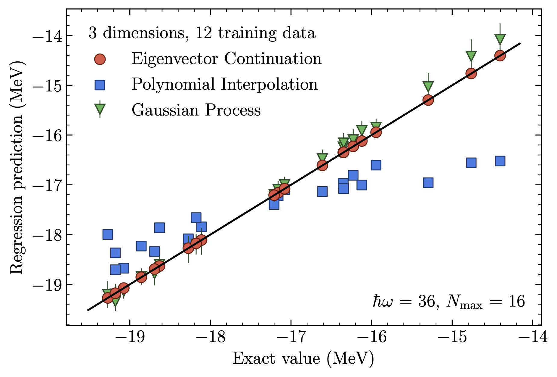
Fig. 34.2 Superior eigenvector continuation emulator accuracy for the ground-state energy of \(^{4}\)He compared to a Gaussian process emulator and conventional interpolation.#
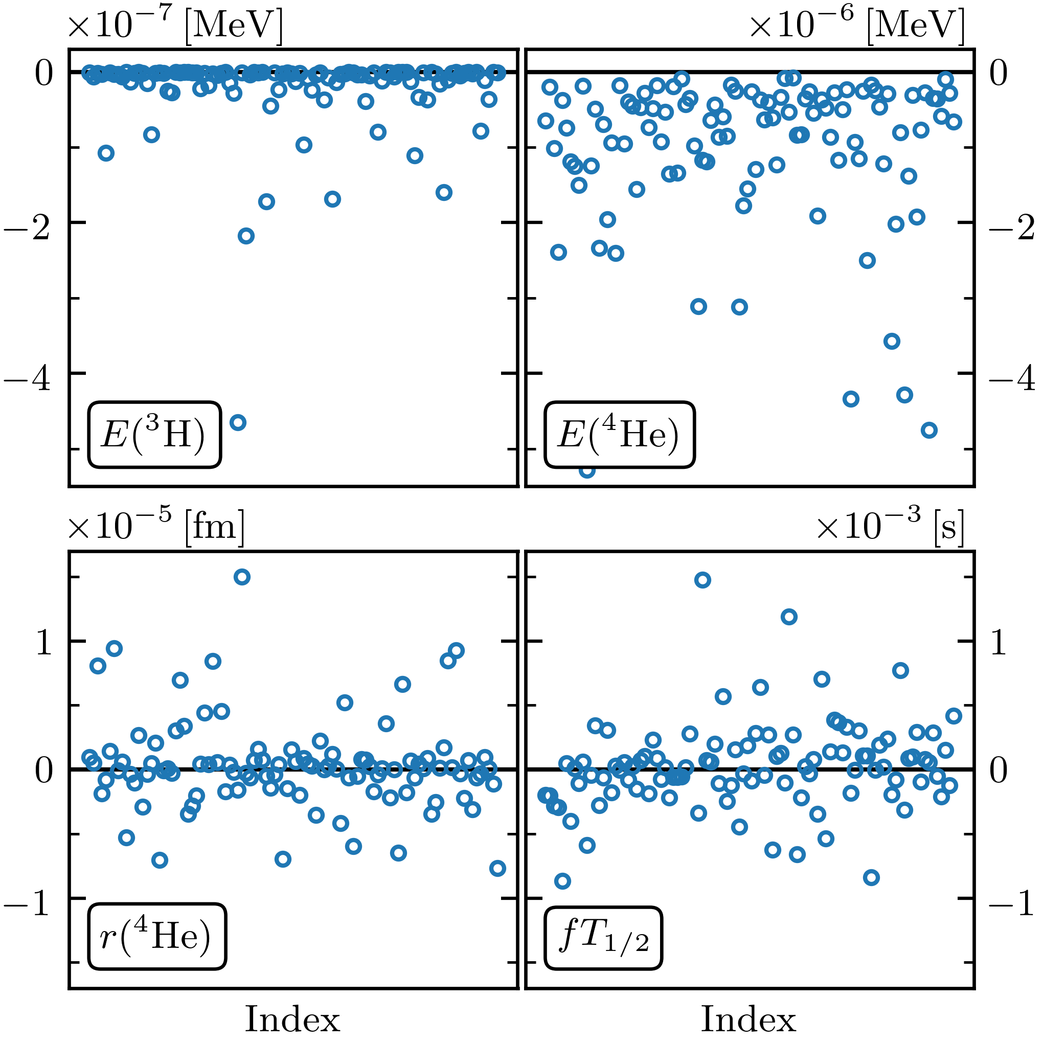
Fig. 34.3 Residuals for four observables from an EC emulator (ground-state energies for \(^3\)H and \(^4\)He, the radius of \(^4\)He, and the \(^3\)H \(\beta\)-decay rate).#
When the offline-online workflow (see Fig. 34.4 for an example) is applied to calculate observables for many parameters characterizing Hamiltonians or other operators, the EC emulators can achieve tremendous speed-ups over high-fidelity computational methods. These gains increase with more difficult calculations; the speed-up for the light nucleus in Fig. 34.2 was over \(10^{5}\) while for coupled cluster calculations of heavy nuclei and nuclear matter speed-ups of order \(10^{9}\) are reported. This facilitates large-scale parameter exploration and calibration as well as sensitivity analyses and experimental design that would otherwise be infeasible. The model-driven nature of the EC approach ensures not only accurate interpolation in the parameter space, but in many cases provides accurate extrapolations in the spaces of control parameters such as coupling strengths, energies, and boundary conditions. A consequence is that problems that are difficult or even intractable for some range of control parameters can be attacked by calculating in a range that can be more easily solved, and then extrapolating using the emulator.
Details#
To start we consider emulators for bound states. Consider a family of matrix Hamiltonians \(H(\pars)\) that depends analytically on some vector of control parameters \(\pars\), which we write in vector notation. We assume that the matrix Hamiltonians are Hermitian for all real values of the parameters. One important example is the affine case where the dependence on each parameter decomposes as a sum of terms
for some functions \(f_\alpha\) and Hermitian matrices \(H_\alpha\). Chiral EFT Hamiltonians, with \(\pars\) being the LECs, are an important example.
Note
It is important to recognize that we do not seek a full spectrum or even more than one or two eigenvalues.
We will be interested in the properties of some particular eigenvector of \(H(\pars)\) and its corresponding eigenvalue \(E(\pars)\),
The basic idea of eigenvector continuation is that \(\ket{\psi(\pars)}\) is an analytic function for real values \(\pars\), and the smoothness implies that it approximately lies on a linear subspace with a finite number of dimensions (see Fig.~\ref{fig:schematic_rbm} for a schematic representation). We note that if there are exact eigenvalue degeneracies, the relative ordering of eigenvalues may change as we vary \(\pars\). However, the eigenvectors can still be defined as analytic functions in the neighborhood of these exact level crossings. The smoother and more gradual the undulations in the eigenvectors, the fewer dimensions needed. A good approximation to \(\ket{\psi(\pars)}\) can be found efficiently using a variational subspace composed of snapshots of \(\ket{\psi(\pars_i)}\) for parameter values \(\pars_i\). We note that for complex values of the parameters, the guarantee of smoothness no longer holds.
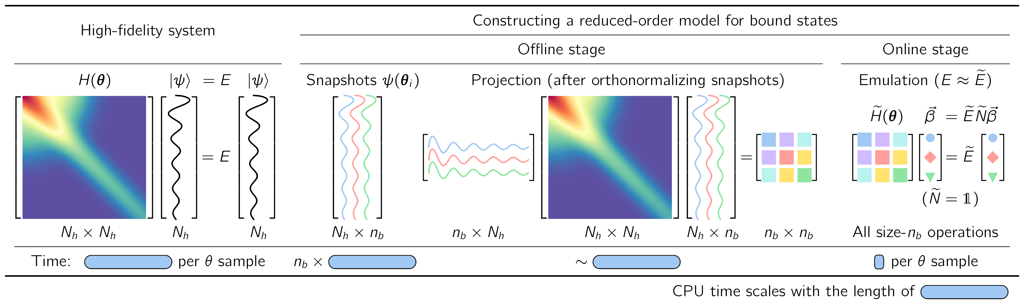
Fig. 34.4 Illustration of the workflow for implementing fast & accurate emulators, including a high-fidelity solver (left) and an intrusive, projection-based emulator with efficient offline-online decomposition (right), for sampling the (approximate) solutions of the Schrodinger equation in the parameter space \(\pars\).#
The basic ingredients of an RBM workflow, which is built on a separation into offline and online stages, are illustrated for a familiar Hamiltonian eigenvalue problem in Fig. 34.4.
Formulation in integral form. First we cast the equations for the Schrodinger wave function or other quantities of interest (such as a scattering matrix) in integral form. For the Hamiltonian eigenvalue problem in Fig. 34.4 (left) with parameters \(\pars\), solving the finite matrix problem of a (large) basis size \(N_h\times N_h\) is formally equivalent to finding \(N_h\) (approximate) stationary solutions to the variational functional
in the space spanned by the \(N_h\) basis elements. This is our high-fidelity model.
Offline stage. Next we reduce the dimensionality of the problem by substituting for the general solution a trial basis of size \(\nb\). RBMs start with a snapshot basis, consisting of high-fidelity solutions \(\ket{\psi_i}\) at selected values \(\{\pars_i;\, i=1,\ldots,n_b\}\) in the parameter space, as in Fig. 34.4 (right). When seeking the ground state energy and wave function for arbitrary \(\pars\), these \(\ket{\psi_i}\) are ground-state eigenvectors from diagonalizing \(H(\pars_i)\). For many EC applications in nuclear physics it has been sufficient to choose this basis randomly, e.g., with a space-filling sampling algorithm such as Latin hypercube sampling. This basis spans a reduced space and can be used directly (after orthonormalizing the snapshots),
with basis expansion coefficients \(\beta_i\). The Hamiltonian is then projected to a much smaller \(\nb\times\nb\) space, as shown in Fig. 34.4b and schematically in Fig. 34.5.
More generally in RBM applications, one first compresses the snapshot basis by applying some variation of principal component analysis (known as proper orthogonal decomposition or POD in this context), which builds on the singular value decomposition (SVD) of the snapshots and enables a smaller basis size than \(n_b\). Alternatively, or in conjunction with POD, one can efficiently select snapshots by applying an active learning protocol (greedy algorithm) that aims to minimize the overall error of the emulator.
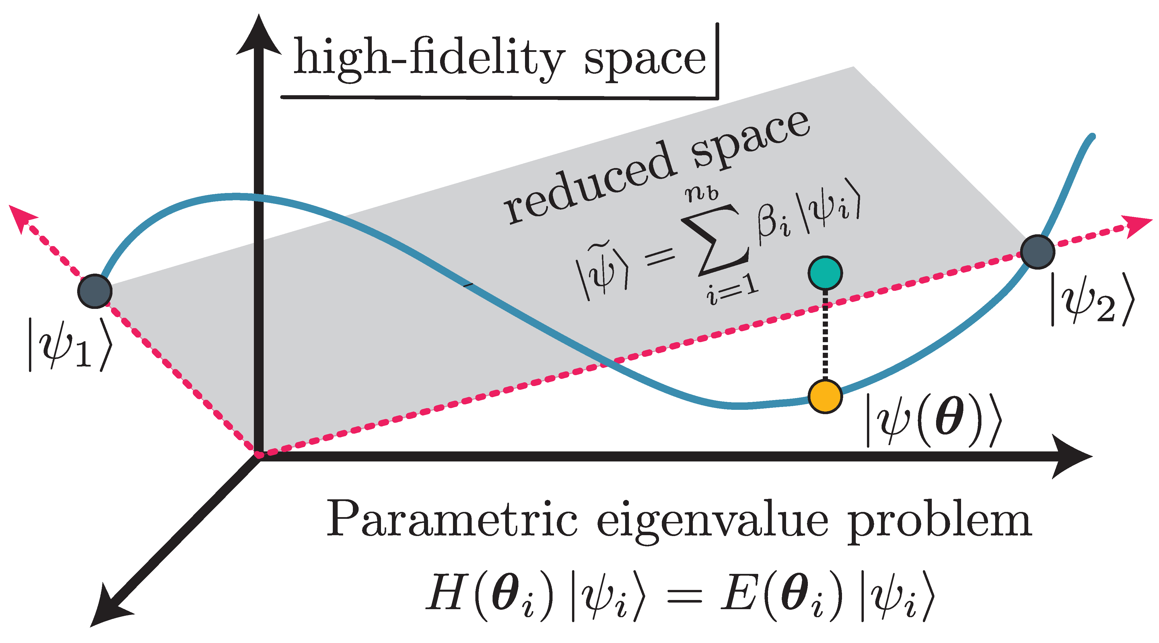
Fig. 34.5 Schematic RBM representation.]{Schematic RBM representation. The high-fidelity trajectory in the Hilbert space is in blue, and include two high-fidelity snapshots (\(\pars_1\) and \(\pars_2\)), which span the ROM subspace (grey). Subspace projection is shown for \(\ket{\psi(\pars)}\).#
Online stage. For variational formulations, we enforce stationarity with respect to the trial basis expansion coefficients. This leads to a \(\nb\times\nb\) generalized eigenvalue problem for the basis coefficients,
as visualized in Fig. 34.4 (right). Note that if the basis has been orthonormalized, then \(\wt N\) is an identity matrix. Extending such an emulator to matrix elements of other operators and even transitions is straightforward.
Comparison of variational and Galerkin emulators#
The variational method formulates the solution to an eigenvalue problem as a stationary functional as in (34.8). Upon inserting a trial basis as in (34.9), we obtain a generalized eigenvalue problem, (34.10).
In the Galerkin approach, we start with the weak form arising from multiplying the underlying equations and boundary conditions by arbitrary test functions and integrating over the relevant domains.
The Galerkin approach starts with the schematic form
with arbitrary test functions \(\ket{\zeta}\). The reduced dimensionality for Galerkin RBM formulations enforces orthogonality with a restricted set of \(\nb\) test functions,
If the test functions are chosen to be the trial basis functions, \(\bra{\zeta_i} = \bra{\psi_i}\), then this is called Bubnov-Galerkin or Ritz-Galerkin (or just Galerkin). If a different basis of test functions is used, this is called Petrov-Galerkin. For eigenvalue problems with Hamiltonians that are bounded from below, the Ritz-Galerkin procedure yields the same equations as the variational approach. The Petrov-Galerkin option means that the Galerkin procedure is more general.
In uncertainty quantification, for which sampling of very many parameter sets are usually required, it is essential that the emulator be many times faster than the high-fidelity calculations. This is achieved for RBM emulators by the offline and online separation because the online stage only requires computations scaling with \(\nb\) (small) and not \(N_h\) (large). An affine operator structure, meaning a factorization of parameter dependence as in (34.7), is needed to achieve the desired online efficiency because size-\(N_h\) operations such as \(\mel{\psi_i}{H_\alpha}{\psi_j}\) are independent of \(\pars\) and only need to be calculated once in the offline stage. If the problem is non-affine, then the strategy is to apply a so-called hyperreduction approach, which leads to an approximate affine form.
EC applications#
The application of EC has been widespread in low-energy nuclear physics and is spreading beyond. The applications include (see review article on EC:
ground-state properties (energies, radii), excited states, and resonances;
transition matrix elements;
pairing; shell model;
special versions for the coupled cluster approach and MBPT;
systems in a finite box
subspace diag. on quantum computers
extensions to non-eigen-value problems: reactions and scattering; fission.
The extensions to scattering problems initially used the Kohn Variational Principle, but were quickly extended to variational methods based on scattering matrices rather than wave functions. Galerkin methods have generalized all these results.