32.6. Expansion parameter#
At a large but finite width, the distribution over output functions acquires non-Gaussian components, but the near-CLT averaging enables these correlations to be treated in a controlled manner. At the same time, increasing depth \(\ell_{out}\) introduces increasing correlations. These opposing tendencies lead to the identification of the ratio \(r \equiv \ell_{out}/n\) being significant as both \(n\) and \(\ell_{out}\) become large. \(r\) acts as an expansion parameter that suppresses higher-order, non-Gaussian correlations in the limit of small \(r\).
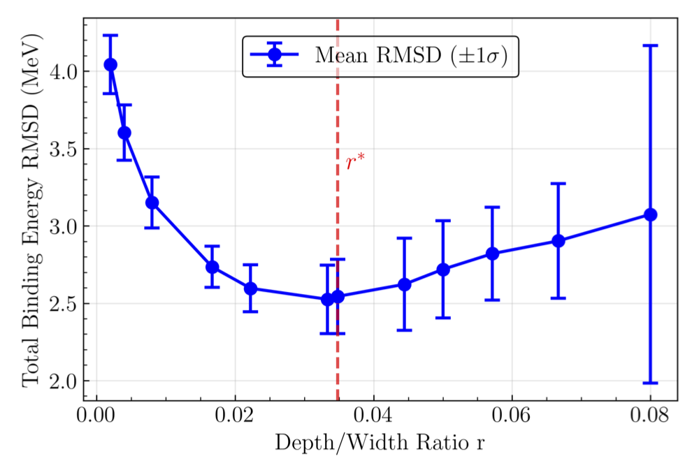
Fig. 32.13 The mean root-mean-square (rms) deviation of the binding energy data and the two-input-network outputs for \(100\) trainings vs. ratio of depth-to-width \(r\), with the depth \(\ell_{out} = 4\). Trainings with binding-energy RMSD\(\geq30\) MeV were omitted from calculation of the mean value of the binding-energy RMSD. The red horizontal line is the \(r^*\) value for this network, calculated to be \(r^*=0.034\). This labels the cutoff where the effectively deep regime begins to transition into the chaotic regime with increasing \(r\).#
As an expansion parameter, \(r\) quantifies the degree of correlation between neurons in a network. This results in three regimes describing the initialized output distribution:
\(r\rightarrow0\), all terms in the action dependent on \(r\) vanish, and the output distribution becomes Gaussian (effectively infinite width, CLT kicks in). These networks have turned off their correlations.
\(0 < r \ll 1\), the moments are controllable, truncated, and nontrivial, as is desired in our effective theory approach. These networks are in what is known as the “effectively deep” regime.
\(r\geq1\), the moments are strongly coupled, and every term in the \(r\) expansion contributes to the action. In this regime, the theory becomes highly non-perturbative, and an effective description becomes impossible.
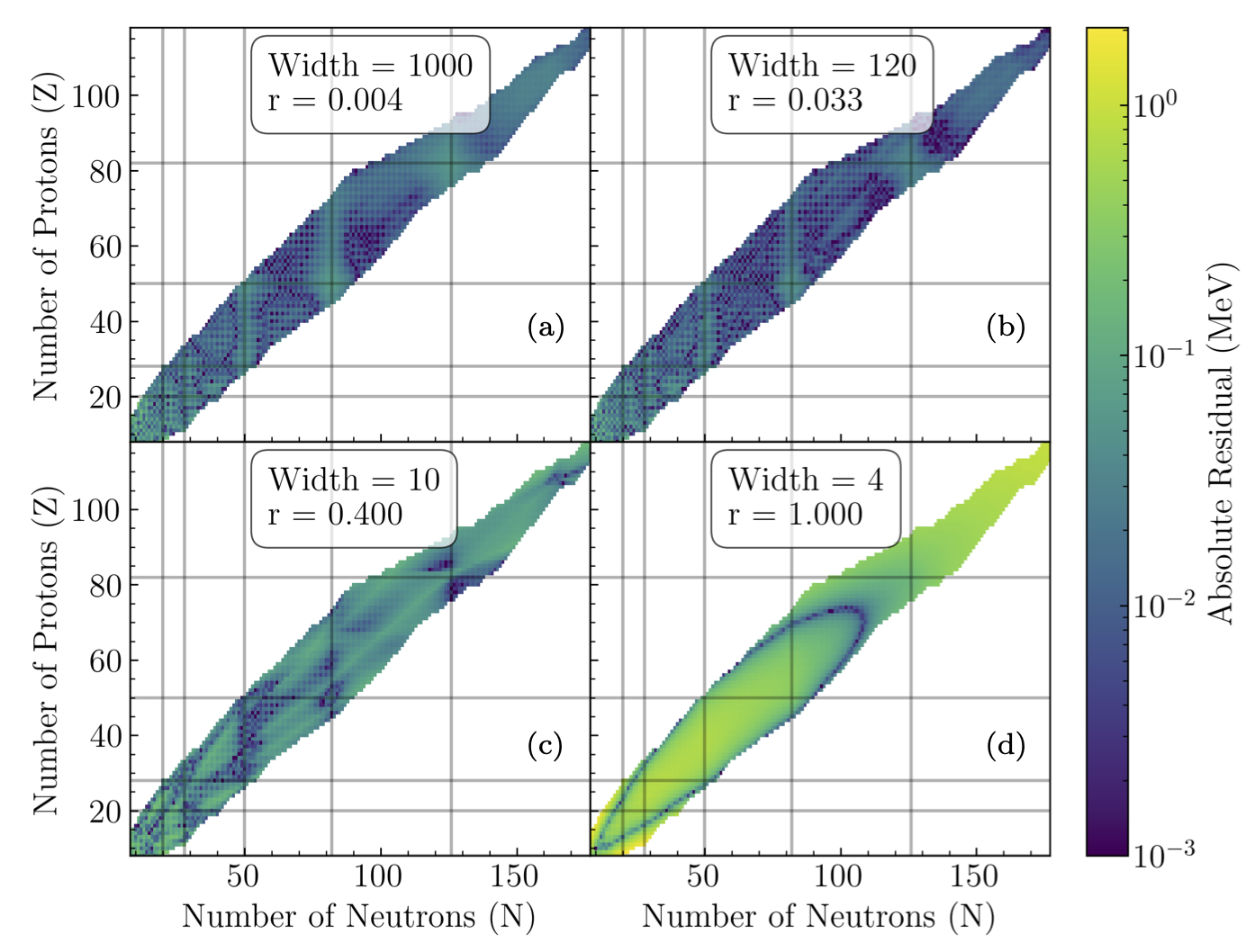
Fig. 32.14 Residual plots for a trained 2 input binding energy network with a fixed depth of 4, and widths of (a) 4, (b) 10, (c) 120, and (d) 1000 to demonstrate the different learning regimes in ANNFT.#
The four plots correspond to different regimes:
\(r=0.004\): Still able to learn, but will only learn more trivially as \(r\rightarrow 0\). Mean BE RMSD of 3.6 MeV.
\(r = 0.033\): The most learning-capable critical network. Mean BE RMSD of 2.52 MeV.
\(r = 0.4\): Loses feature learning to more strongly correlated neurons as \(r\rightarrow 1\). Mean BE RMSD of 56 MeV (bimodal between 72 and \(\sim\)3 MeV).
\(r = 1.0\): Neuron correlations prevent any learning beyond the simplest loss local minima. Mean BE RMSD of 72 MeV.