8.5. BLR-III: Demo

Prelude: ordinary linear regression

To warm up, and get acquainted with the notation and formalism, let us work out a small example. Assume that we have the situation where we have collected two datapoints \(\data = [y_1,y_2]^T = [-3,3]^T\) for the predictor values \([x_1,x_2]^T = [-2,1]^T\).

This data could have come from any process, even a non-linear one. But this is artificial data that I generated by evaluating the function \(y = 1 + 2x\) at \(x=x_1=-2\) and \(x=x_2=1\). Clearly, the data-generating mechanism is very simple and corresponds to a linear model \(y = \paraLR_0 + \paraLR_1 x\) with \([\paraLR_0,\paraLR_1] = [1,2]\). This is the kind of information we never have in reality. Indeed, we are always uncertain about the process that maps input to output, and as such our model \(M\) will always be wrong. We are also uncertain about the parameters \(\parsLR\) of our model. These are the some of the fundamental reasons for why it can be useful to operate with a Bayesian approach where we can assign probabilities to any quantity and statement. In this example, however, we will continue with the standard (frequentist) approach based on finding the parameters that minimize the squared errors (i.e., the norm of the residual vector).

We will now assume a linear model with polynomial basis up to order one to model the data, i.e.,

\[ M(\parsLR;\inputt) = \paraLR_0 + \paraLR_1 \inputt, \]

which we can express in terms of a design matrix \(\dmat\) and (unknown) parameter vector \(\parsLR\) as \(M = \dmat \parsLR\).

In the present case the two unknowns \(\parsLR = [\paraLR_0,\paraLR_1]^T\) can be fit to the two datapoints \(\data = [-3,3]^T\) using pen a paper.

Exercise 8.5

In the example above you have two data points and two unknowns, which means you can easily solve for the model parameters using a conventional matrix inverse. Do the numerical calculation to make sure you have set up the problem correctly.

Exercise 8.6

Evaluate the normal equations for the design matrix \(\dmat\) and data vector \(\data\) in the example above.

Exercise 8.7

Evaluate the sample variance \(s^2\) for the example above using Eq. (8.24). Do you think the result makes sense?

Continuing …

For the time being we assume to know enough about the data to consider a normal likelihood with i.i.d. errors. Let us first set the known residual variance to \(\sigmares^2 = 0.5^2\).

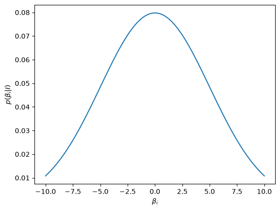
This time we also have prior knowledge that we would like to build into the inference. Here we use a normal prior for the parameters with \(\sigma_\paraLR = 5.0\), which is to say that before looking at the data we believe the pdf for \(\parsLR\) to be centered on zero with a variance of \(5^2\).

Let us plot this prior. The prior is the same for \(\paraLR_0\) and \(\paraLR_1\), so it is enough to plot one of them.

import numpy as np
import matplotlib.pyplot as plt
from scipy.stats import norm

def normal_distribution(mu,sigma2):
    return norm(loc=mu,scale=np.sqrt(sigma2))

betai = np.linspace(-10,10,100)
prior = normal_distribution(0,5.0**2)

fig, ax = plt.subplots(1,1)
ax.plot(betai,prior.pdf(betai))
ax.set_ylabel(r'$p(\beta_i \vert I )$')
ax.set_xlabel(r'$\beta_i$');

It is straightforward to evaluate Eq. (8.42), which gives us

(8.47)\[\begin{split} \tildecovparsLR^{-1} &= 4 \begin{pmatrix} 2.01 & -1.0 \\ -1.0 & 5.01 \end{pmatrix} \\ \tilde{\parsLR} &= ( 0.992, 1.994) \end{split}\]

This should be compared with the parameter vector \((1,2)\) we recovered using ordinary linear regression. With Bayesian linear regression we start from an informative prior with both parameters centered on zero with a rather large variance.

Exercise 8.8 (Warm-up Bayesian linear regression)

Reproduce the posterior mean and covariance matrix from Eq. (8.47). You can use numpy methods to perform the linear algebra operations.

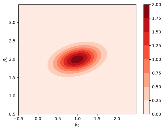
We can plot the posterior probability distribution for \(\pars\), i.e., by plotting the bi-variate \(\mathcal{N}-\)distribution with the parameter in Eq. (8.47).

from scipy.stats import multivariate_normal

mu = np.array([0.992,1.992])
Sigma = np.linalg.inv(4 * np.array([[2.01,-1.0],[-1.0,5.01]]))

posterior = multivariate_normal(mean=mu, cov=Sigma)

beta0, beta1 = np.mgrid[-0.5:2.5:.01, 0.5:3.5:.01]
beta_grid = np.dstack((beta0, beta1))

fig,ax = plt.subplots(1,1)
ax.set_xlabel(r'$\beta_0$')
ax.set_ylabel(r'$\beta_1$')
im = ax.contourf(beta0, beta1, posterior.pdf(beta_grid),cmap=plt.cm.Reds);
fig.colorbar(im);

Using Eq. (8.44) we can obtain, e.g., the \(\paraLR_1\) marginal density and compare with the prior

beta1 = np.linspace(-0.5,4.5,200)
mu1 = mu[1]
Sigma11_sq = Sigma[1,1]

posterior1 = normal_distribution(mu1,Sigma11_sq)

fig, ax = plt.subplots(1,1)
ax.plot(beta1,posterior1.pdf(beta1),'r-',\
label=r'$p(\beta_1 \vert \mathcal{D}, \sigma_\epsilon^2, I )$')
ax.plot(beta1,prior.pdf(beta1), 'b--',label=r'$p(\beta_1 \vert I )$')
ax.set_ylabel(r'$p(\beta_1 \vert \ldots )$')
ax.set_xlabel(r'$\beta_1$')
ax.legend(loc='best');

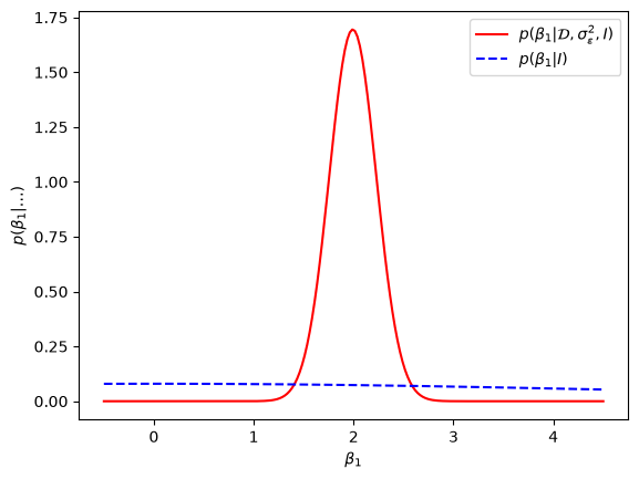
The key take-away with this numerical exercise is that Bayesian inference yields a probability distribution for the model parameters whose values we are uncertain about. With ordinary linear regression techniques you only obtain the parameter values that optimize some cost function, and not a probability distribution.

Exercise 8.9 (Warm-up Bayesian linear regression (data errors))

Explore the sensitivity to changes in the residual errors \(\sigmares\). Try to increase and reduce the error.

Exercise 8.10 (Warm-up Bayesian linear regression (prior sensitivity))

Explore the sensitivity to changes in the Gaussian prior width \(\sigma_\paraLR\). Try to increase and reduce the width.

Exercise 8.11 (“In practice” Bayesian linear regression)

Perform Bayesian Linear Regression on the data that was generated in Addendum: Ordinary linear regression in practice. Explore:

• Dependence on the quality of the data (generate data with different \(\sigma_\epsilon\)) or the number of data.

• Dependence on the polynomial function that was used to generate the data.

• Dependence on the number of polynomial terms in the model.

• Dependence on the parameter prior.

In all cases you should compare the Bayesian inference with the results from Ordinary Least Squares and with the true parameters that were used to generate the data.

Solutions to selected exercises

Solution to Exercise 8.5

We have the following design matrix

\[\begin{split} \dmat = \left[ \begin{array}{cc} 1 & -2 \\ 1 & 1 \end{array} \right], \end{split}\]

which in the present case yields the parameter values

\[ \pars^{*} = \dmat^{-1}\data = [1,2]^T. \]

Solution to Exercise 8.7

For the warmup case we have fitted a straight line through two data points, which is always possible, and we cannot determine the sample variance. This will be even more clear when we come to BLR-I: Background.