34.6. Parametric Matrix Model emulators

Overview of PMMs

Parametric Matric Models (PMMs) can be considered a hybrid approach: they are data driven but incorporate model structure so they are in part model driven. Fig. 34.14 provides a schematic overview of PMMs, which we flesh out in the example that follows.

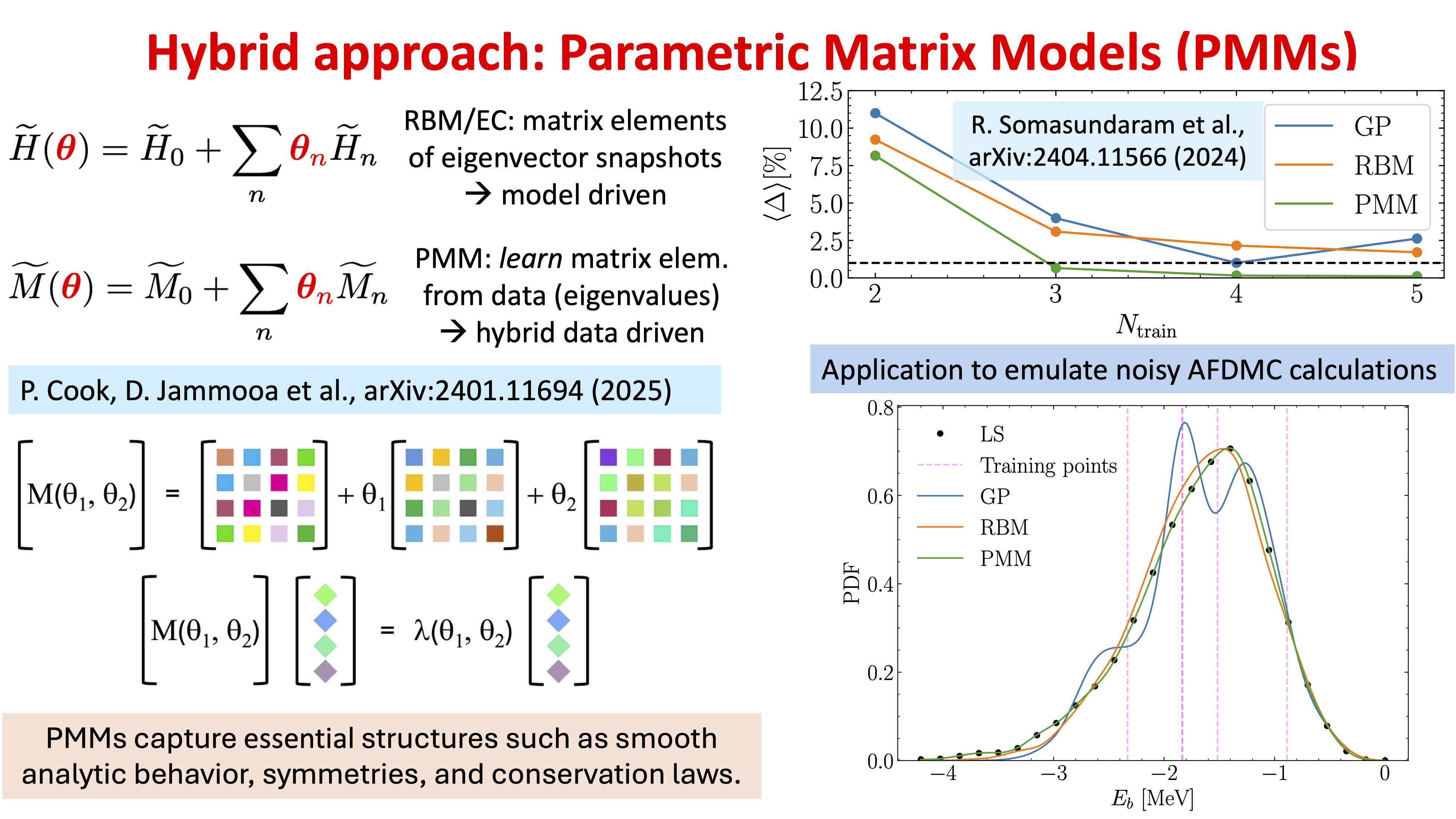
Fig. 34.14 Basic structure of PMM emulation compared to RBM/EC emulation with an example showing the relative performance between RBM, PMM and Gaussian Process (GP) emulator.

Demo: simple example of a PMM emulator

The example below demonstrates how a parametric matrix model (PMM) can be used as an emulator for a more expensive model, and how it compares with eigenvector continuation (EC). [Note: this example and much of the commentary originated with ChatGPT 5.5.]

The basic idea is to replace an expensive calculation with a much smaller matrix model whose eigenvalues reproduce the desired observable.

Details of the example

1. The “expensive” model

The demonstration example defines a larger parameter-dependent Hamiltonian, \(H_{\rm true}(x)\), where \(x\) is an input parameter. In this case, the Hamiltonian \(H_{\rm true}\) is construction as a matrix with dimension \(40 \times 40\). (In an exercise you can modify the code to try a different matrix.) The observable we want to emulate is the ground-state energy,

\[ E_0(x) = \lambda_{\min}\!\left[H_{\rm true}(x)\right], \]

where \(\lambda_{\min}\) is the lowest eigenvalue. In practice we use numpy.linalg.eigvalsh to find the eigenvalue.

In a real application, solving \(H_{\rm true}(x)\) could represent doing a large-scale diagonalization, applying an expensive many-body method, or doing a high-fidelity numerical simulation.

2. Generating training data

The expensive model is evaluated at at a small number of parameter values (in this case 9) in the interval \(x_i \in [-2,2]\), and stores the corresponding outputs as \(y_i = E_0(x_i)\). These points form the training data,

\[ \{(x_i, y_i)\}. \]

The emulator is trained only on this sparse set of points. It is then tested on a denser grid (interpolation), including points outside the training region (extrapolation).

3. The PMM emulator

The PMM emulator is a smaller matrix,

\[ P(x;\theta) = A_0 + x A_1 + x^2 A_2, \]

where \(A_0\), \(A_1\), and \(A_2\) are real symmetric matrices that are to be learned. In the coded example, \(P(x;\theta)\) is only \(4 \times 4\), much smaller than the \(40 \times 40\) truth model. The parameters \(\theta\) are the independent entries of the symmetric matrices \(A_0\), \(A_1\), and \(A_2\). These entries are adjusted during training.

Note that the PMM prediction is not a directly fitted scalar polynomial. Instead, the prediction is the lowest eigenvalue of the learned matrix:

\[ \widehat{E}_0(x;\theta) = \lambda_{\min}\!\left[P(x;\theta)\right]. \]

Thus the predicted scalar output is obtained implicitly through a small eigenvalue problem.

4. Training the PMM

The PMM is trained by minimizing a loss function \(\mathcal{L}(\theta)\), which is the difference between the PMM eigenvalue and the training data:

\[ \mathcal{L}(\theta) = \sum_i \left[ \widehat{E}_0(x_i;\theta) - y_i \right]^2. \]

In the code, this is done using a nonlinear least squares optimizer. Because the eigenvalues depend nonlinearly on the matrix entries, the optimization problem is nonlinear even though the matrix elements themselves are simple polynomials in \(x\). Multiple random restarts are used to reduce the chance of finding a poor local minimum.

5. Why this is different from polynomial regression

The code also fits an ordinary scalar polynomial,

\[ p(x) = c_0 + c_1 x + c_2 x^2 + \cdots. \]

which serves as a baseline comparison.

The polynomial model fits the observable directly as a scalar function of \(x\). By contrast, the PMM fits a matrix whose eigenvalue gives the observable. This distinction matters because eigenvalues of parameter-dependent matrices can produce complicated nonlinear behavior, including avoided-crossing-like curvature and rapid changes in slope. So even if the matrix elements of \(P(x;\theta)\) are only low-order polynomials, the eigenvalues of \(P(x;\theta)\) can have a richer functional structure than an ordinary low-order scalar polynomial.

6. Interpolation and extrapolation

The training data are generated only in the interval \(-2 \le x \le 2\) while the model is then tested on a wider interval \(-3 \le x \le 3\). This separates the test region into two parts:

• Interpolation region: \(-2 \le x \le 2\)

• Extrapolation region: \(x < -2\) or \(x > 2\)

The code reports root-mean-square errors in both regions for the PMM, eigenvector continuation, and the polynomial baseline. This allows one to see whether the emulator is merely fitting the training region or whether it also captures useful structure outside the training domain.

Show code cell source

Hide code cell source

"""
pmm_emulator_with_ec_demo.py

Demonstration of a Parametric Matrix Model (PMM) used as an emulator,
with comparison to eigenvector continuation (EC) and scalar polynomial
regression.

Truth model:
    A moderately large matrix H_true(x), whose lowest eigenvalue E0(x)
    represents an "expensive" observable.

PMM emulator:
    A small trainable symmetric matrix

        P(x) = A0 + x A1 + x^2 A2

    The PMM prediction is the lowest eigenvalue of P(x).

Eigenvector continuation:
    Uses exact ground-state eigenvectors of H_true(x) at the training
    points to build a reduced basis. Then it projects H_true(x) into
    that subspace and diagonalizes the projected Hamiltonian.

The script:
    1. Generates sparse training data from the truth model.
    2. Fits a small PMM to the scalar training data.
    3. Builds an EC emulator from training eigenvectors.
    4. Fits a scalar polynomial regression baseline.
    5. Compares all predictions on a dense test grid.
    6. Plots predictions and semi-log absolute errors.
"""

import numpy as np
import matplotlib.pyplot as plt
from scipy.optimize import least_squares


# ----------------------------------------------------------------------
# Utilities
# ----------------------------------------------------------------------

def symmetric_from_params(params, n):
    """
    Construct a real symmetric n x n matrix from n(n+1)/2 parameters.
    """
    M = np.zeros((n, n))
    k = 0

    for i in range(n):
        for j in range(i, n):
            M[i, j] = params[k]
            M[j, i] = params[k]
            k += 1

    return M


def unpack_pmm_params(theta, n_pmm, degree):
    """
    Convert a parameter vector theta into matrices A0, A1, ..., A_degree.
    """
    n_tri = n_pmm * (n_pmm + 1) // 2
    matrices = []

    for d in range(degree + 1):
        block = theta[d * n_tri : (d + 1) * n_tri]
        matrices.append(symmetric_from_params(block, n_pmm))

    return matrices


def pmm_matrix(x, theta, n_pmm=4, degree=2):
    """
    Construct the PMM matrix

        P(x) = A0 + x A1 + x^2 A2 + ...
    """
    matrices = unpack_pmm_params(theta, n_pmm, degree)

    P = np.zeros((n_pmm, n_pmm))

    for d, A in enumerate(matrices):
        P += (x**d) * A

    return P


def pmm_predict_one(x, theta, n_pmm=4, degree=2, eigen_index=0):
    """
    Predict using one eigenvalue of the PMM matrix.

    eigen_index=0 means the lowest eigenvalue.
    """
    evals = np.linalg.eigvalsh(pmm_matrix(x, theta, n_pmm, degree))
    return evals[eigen_index]


def pmm_predict(x_values, theta, n_pmm=4, degree=2, eigen_index=0):
    """
    Vectorized PMM prediction.
    """
    return np.array([
        pmm_predict_one(x, theta, n_pmm, degree, eigen_index)
        for x in x_values
    ])


# ----------------------------------------------------------------------
# A synthetic "expensive" truth model
# ----------------------------------------------------------------------

def make_truth_matrices(n_true=40, seed=123):
    """
    Build fixed matrices defining the truth Hamiltonian.

        H_true(x) = H0 + x V + x^2 W + nonlinear diagonal term

    The nonlinear diagonal term makes the target smooth but nontrivial.
    """
    rng = np.random.default_rng(seed)

    def rand_sym(scale):
        A = rng.normal(scale=scale, size=(n_true, n_true))
        return 0.5 * (A + A.T)

    H0 = rand_sym(0.5)
    V = rand_sym(0.25)
    W = rand_sym(0.08)

    # Structured diagonal part, which gives smooth but non-polynomial
    # parameter dependence through the sin(1.5 x) prefactor.
    grid = np.linspace(-2.0, 2.0, n_true)
    D = np.diag(grid**2)

    return H0, V, W, D


H0_TRUE, V_TRUE, W_TRUE, D_TRUE = make_truth_matrices()


def H_true(x):
    """
    The larger, more expensive model.
    """
    return (
        H0_TRUE
        + x * V_TRUE
        + x**2 * W_TRUE
        + 0.15 * np.sin(1.5 * x) * D_TRUE
    )


def expensive_observable(x):
    """
    Observable to emulate: the ground-state energy of H_true(x).
    """
    return np.linalg.eigvalsh(H_true(x))[0]


def expensive_observable_array(x_values):
    """
    Vectorized expensive observable.
    """
    return np.array([expensive_observable(x) for x in x_values])


# ----------------------------------------------------------------------
# Eigenvector continuation emulator
# ----------------------------------------------------------------------

def build_ec_basis(x_train, svd_tol=1e-10):
    """
    Build an eigenvector-continuation basis from exact ground-state
    eigenvectors of the truth Hamiltonian at the training points.

    Parameters
    ----------
    x_train : array
        Training parameter values.
    svd_tol : float
        Relative cutoff for discarding nearly linearly dependent EC basis
        directions.

    Returns
    -------
    Q : array, shape (n_true, n_ec)
        Orthonormal EC basis vectors as columns.
    overlap_evals : array
        Eigenvalues of the raw overlap matrix B.T @ B.
    """
    basis_vectors = []

    for x in x_train:
        evals, evecs = np.linalg.eigh(H_true(x))
        psi0 = evecs[:, 0]
        basis_vectors.append(psi0)

    # Raw nonorthogonal EC basis: columns are training eigenvectors.
    B = np.column_stack(basis_vectors)

    # Canonical orthonormalization of the nonorthogonal basis.
    S = B.T @ B
    s, U = np.linalg.eigh(S)

    keep = s > svd_tol * np.max(s)

    if np.sum(keep) == 0:
        raise RuntimeError("EC basis is numerically singular.")

    Q = B @ U[:, keep] @ np.diag(1.0 / np.sqrt(s[keep]))

    return Q, s


def ec_predict_one(x, Q):
    """
    Eigenvector-continuation prediction at one x.

    The full Hamiltonian is projected into the EC subspace:

        H_EC(x) = Q.T @ H_true(x) @ Q

    and the EC prediction is its lowest eigenvalue.
    """
    H_proj = Q.T @ H_true(x) @ Q
    return np.linalg.eigvalsh(H_proj)[0]


def ec_predict(x_values, Q):
    """
    Vectorized EC prediction.
    """
    return np.array([ec_predict_one(x, Q) for x in x_values])


# ----------------------------------------------------------------------
# Fit the PMM emulator
# ----------------------------------------------------------------------

def fit_pmm(
    x_train,
    y_train,
    n_pmm=4,
    degree=2,
    eigen_index=0,
    seed=1234,
    n_restarts=30,
    max_nfev=5000,
):
    """
    Fit the PMM by nonlinear least squares.

    Because eigenvalue models are nonlinear in the matrix entries,
    multiple random restarts are useful.
    """
    rng = np.random.default_rng(seed)

    n_tri = n_pmm * (n_pmm + 1) // 2
    n_params = (degree + 1) * n_tri

    best_result = None
    best_loss = np.inf

    y_scale = np.std(y_train)
    if y_scale == 0.0:
        y_scale = 1.0

    def residuals(theta):
        y_pred = pmm_predict(
            x_train,
            theta,
            n_pmm=n_pmm,
            degree=degree,
            eigen_index=eigen_index,
        )
        return (y_pred - y_train) / y_scale

    for restart in range(n_restarts):
        theta0 = rng.normal(scale=0.2, size=n_params)

        result = least_squares(
            residuals,
            theta0,
            max_nfev=max_nfev,
            xtol=1e-11,
            ftol=1e-11,
            gtol=1e-11,
        )

        loss = np.mean(residuals(result.x)**2)

        if loss < best_loss:
            best_loss = loss
            best_result = result

    return best_result.x, best_loss


# ----------------------------------------------------------------------
# Polynomial baseline
# ----------------------------------------------------------------------

def fit_polynomial_baseline(x_train, y_train, degree=6):
    """
    Ordinary scalar polynomial regression baseline.
    """
    coeffs = np.polyfit(x_train, y_train, degree)
    return coeffs


def polynomial_predict(x_values, coeffs):
    """
    Evaluate scalar polynomial baseline.
    """
    return np.polyval(coeffs, x_values)


# ----------------------------------------------------------------------
# Error metrics
# ----------------------------------------------------------------------

def rmse(y_pred, y_true):
    """
    Root-mean-square error.
    """
    return np.sqrt(np.mean((y_pred - y_true)**2))


# ----------------------------------------------------------------------
# Main demo
# ----------------------------------------------------------------------

def run_demo(
    n_pmm=4,
    pmm_degree=2,
    poly_degree=6,
    n_train=13,
    x_train_min=-2.0,
    x_train_max=2.0,
    x_test_min=-3.0,
    x_test_max=3.0,
    n_test=401,
):
    # Training region and test region.
    x_train = np.linspace(x_train_min, x_train_max, n_train)
    x_test = np.linspace(x_test_min, x_test_max, n_test)

    # Generate sparse training data from the expensive model.
    y_train = expensive_observable_array(x_train)
    y_test = expensive_observable_array(x_test)

    # Fit PMM emulator using only scalar training outputs.
    theta_pmm, pmm_train_loss = fit_pmm(
        x_train,
        y_train,
        n_pmm=n_pmm,
        degree=pmm_degree,
        eigen_index=0,
        n_restarts=30,
    )

    y_pmm = pmm_predict(
        x_test,
        theta_pmm,
        n_pmm=n_pmm,
        degree=pmm_degree,
        eigen_index=0,
    )

    # Build EC emulator using training eigenvectors and the true Hamiltonian.
    Q_ec, ec_overlap_evals = build_ec_basis(x_train)
    y_ec = ec_predict(x_test, Q_ec)

    # Fit scalar polynomial baseline.
    poly_degree_eff = min(poly_degree, n_train - 1)
    
    poly_coeffs = fit_polynomial_baseline(
        x_train,
        y_train,
        degree=poly_degree_eff,
    )
    y_poly = polynomial_predict(x_test, poly_coeffs)

    # Error metrics.
    train_mask = (x_test >= x_train_min) & (x_test <= x_train_max)
    extra_mask = ~train_mask

    pmm_rmse_interp = rmse(y_pmm[train_mask], y_test[train_mask])
    pmm_rmse_extra = rmse(y_pmm[extra_mask], y_test[extra_mask])

    ec_rmse_interp = rmse(y_ec[train_mask], y_test[train_mask])
    ec_rmse_extra = rmse(y_ec[extra_mask], y_test[extra_mask])

    poly_rmse_interp = rmse(y_poly[train_mask], y_test[train_mask])
    poly_rmse_extra = rmse(y_poly[extra_mask], y_test[extra_mask])

    print("PMM emulator demo with eigenvector continuation")
    print("-----------------------------------------------")
    print(f"Number of training points:       {len(x_train)}")
    print(f"Truth matrix dimension:          {H0_TRUE.shape[0]}")
    print(f"PMM matrix dimension:            {n_pmm}")
    print(f"PMM polynomial degree:           {pmm_degree}")
    print(f"Polynomial baseline degree:      {poly_degree}")
    print(f"PMM training loss:               {pmm_train_loss:.3e}")
    print(f"EC basis dimension:              {Q_ec.shape[1]}")
    print(f"Smallest raw EC overlap eigval:  {np.min(ec_overlap_evals):.3e}")
    print()

    print("RMSE on dense test grid")
    print(f"  PMM interpolation region:      {pmm_rmse_interp:.3e}")
    print(f"  PMM extrapolation region:      {pmm_rmse_extra:.3e}")
    print(f"  EC interpolation region:       {ec_rmse_interp:.3e}")
    print(f"  EC extrapolation region:       {ec_rmse_extra:.3e}")
    print(f"  Polynomial interpolation:      {poly_rmse_interp:.3e}")
    print(f"  Polynomial extrapolation:      {poly_rmse_extra:.3e}")

    # ------------------------------------------------------------------
    # Plot emulator predictions.
    # ------------------------------------------------------------------
    plt.figure(figsize=(8, 5))

    plt.plot(
        x_test,
        y_test,
        label="Expensive model",
        lw=2.5,
    )

    plt.plot(
        x_test,
        y_pmm,
        "--",
        label="PMM emulator",
        lw=2.0,
    )

    plt.plot(
        x_test,
        y_ec,
        "-.",
        label="Eigenvector continuation",
        lw=2.0,
    )

    plt.plot(
        x_test,
        y_poly,
        ":",
        label="Polynomial baseline",
        lw=2.0,
    )

    plt.scatter(
        x_train,
        y_train,
        label="Training data",
        zorder=5,
    )

    plt.axvspan(x_test_min, x_train_min, alpha=0.08)
    plt.axvspan(x_train_max, x_test_max, alpha=0.08)

    plt.xlabel(r"Input parameter $x$")
    plt.ylabel(r"Observable $E_0(x)$")
    plt.title("PMM emulator compared with EC and polynomial regression")
    plt.legend()
    plt.grid(alpha=0.3)
    plt.tight_layout()
    plt.show()

    # ------------------------------------------------------------------
    # Plot absolute errors on a semi-log scale.
    # ------------------------------------------------------------------
    plt.figure(figsize=(8, 5))

    eps = 1e-14

    plt.semilogy(
        x_test,
        np.abs(y_pmm - y_test) + eps,
        label="PMM absolute error",
        lw=2.0,
    )

    plt.semilogy(
        x_test,
        np.abs(y_ec - y_test) + eps,
        label="EC absolute error",
        lw=2.0,
    )

    plt.semilogy(
        x_test,
        np.abs(y_poly - y_test) + eps,
        label="Polynomial absolute error",
        lw=2.0,
    )

    plt.axvline(x_train_min, lw=1.0, ls="--")
    plt.axvline(x_train_max, lw=1.0, ls="--")

    plt.xlabel(r"Input parameter $x$")
    plt.ylabel(r"Absolute prediction error")
    plt.title("Absolute emulator errors")
    plt.legend()
    plt.grid(alpha=0.3, which="both")
    plt.tight_layout()
    plt.show()

    return {
        "x_train": x_train,
        "y_train": y_train,
        "x_test": x_test,
        "y_test": y_test,
        "y_pmm": y_pmm,
        "y_ec": y_ec,
        "y_poly": y_poly,
        "theta_pmm": theta_pmm,
        "Q_ec": Q_ec,
        "ec_overlap_evals": ec_overlap_evals,
        "poly_coeffs": poly_coeffs,
        "pmm_train_loss": pmm_train_loss,
        "rmse": {
            "pmm_interp": pmm_rmse_interp,
            "pmm_extra": pmm_rmse_extra,
            "ec_interp": ec_rmse_interp,
            "ec_extra": ec_rmse_extra,
            "poly_interp": poly_rmse_interp,
            "poly_extra": poly_rmse_extra,
        },
    }

results = run_demo(n_train=9)

PMM emulator demo with eigenvector continuation
-----------------------------------------------
Number of training points:       9
Truth matrix dimension:          40
PMM matrix dimension:            4
PMM polynomial degree:           2
Polynomial baseline degree:      6
PMM training loss:               3.727e-22
EC basis dimension:              9
Smallest raw EC overlap eigval:  2.562e-05

RMSE on dense test grid
  PMM interpolation region:      3.880e-03
  PMM extrapolation region:      1.389e-01
  EC interpolation region:       3.833e-05
  EC extrapolation region:       2.963e-02
  Polynomial interpolation:      1.010e-02
  Polynomial extrapolation:      9.715e-01

Summary of results

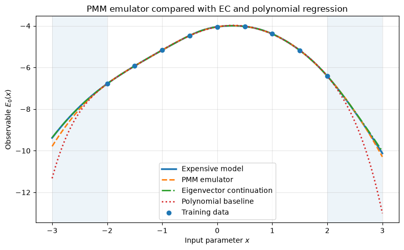
The first plot compares four curves:

1. The expensive model result, \(E_0(x)\)

2. The PMM emulator prediction, \(\widehat{E}_0(x)\)

3. The eigenvector-continuation prediction, \(E_0^{\rm EC}(x)\)

4. The polynomial regression baseline, \(p(x)\)

The training points are shown as markers. The shaded regions indicate extrapolation beyond the training interval. This plot answers the qualitative question:

Does the learned PMM emulator reproduce the expensive model over the test range?

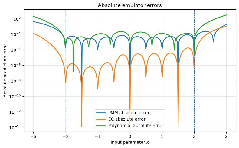
The second plot shows the absolute prediction errors,

\[ \left| \widehat{E}_0(x) - E_0(x) \right|, \]

for the PMM and EC emulators, and the polynomial baseline. Because the vertical axis is logarithmic, the plot can show small and large errors on the same figure. This is useful because emulator errors often vary by orders of magnitude between the interpolation and extrapolation regions. The semi-log plot makes it easier to see where each emulator is accurate, where it fails, and how its error compares with the alternatives.

The PMM part of the demonstration illustrates the main emulator idea:

\[ \text{expensive model} \quad \longrightarrow \quad \text{small learned matrix model} \quad \longrightarrow \quad \text{cheap eigenvalue prediction}. \]

The expensive calculation requires diagonalizing a larger matrix,

\[ H_{\rm true}(x) \in \mathbb{R}^{40 \times 40}, \]

while the PMM emulator only requires diagonalizing a small matrix,

\[ P(x;\theta) \in \mathbb{R}^{4 \times 4}. \]

After training, the PMM provides a fast surrogate for the expensive observable.

The important point is that the PMM does not simply interpolate the observable with an ordinary scalar function. Instead, it learns a small parameter-dependent matrix whose spectral properties mimic the behavior of the target system.

What eigenvector continuation does in this example

Set-up of EC

As described in Section 34.3, eigenvector continuation (EC) is a reduced-basis method for parameter-dependent eigenvalue problems. Let’s review how it is implemented here. Suppose one has a family of Hamiltonians,

\[ H(x), \]

and solves the full problem at selected training points,

\[ x_1, x_2, \ldots, x_m. \]

At each training point one computes an eigenvector, usually the ground-state vector,

\[ |\psi_0(x_i)\rangle. \]

These training eigenvectors (called snapshots) are then used to form a reduced subspace,

\[ \mathcal{S}_{\rm EC} = \mathrm{span} \left\{ |\psi_0(x_1)\rangle, |\psi_0(x_2)\rangle, \ldots, |\psi_0(x_m)\rangle \right\}. \]

In the code, this is done by diagonalizing the full truth Hamiltonian \(H_{\rm true}(x_i)\) at each training point and saving the corresponding ground-state eigenvector.

Projecting the Hamiltonian

Once the EC basis is constructed, the Hamiltonian is projected into this reduced subspace. If the training eigenvectors are denoted by \(|\psi_i\rangle\), where

\[ |\psi_i\rangle \equiv |\psi_0(x_i)\rangle, \]

then the projected Hamiltonian is

\[ H^{\rm EC}_{ij}(x) = \langle \psi_i | H_{\rm true}(x) | \psi_j \rangle. \]

The overlap matrix is

\[ N^{\rm EC}_{ij} = \langle \psi_i | \psi_j \rangle. \]

The EC prediction is obtained by solving the generalized eigenvalue problem

\[ H^{\rm EC}(x)c = E^{\rm EC}(x) N^{\rm EC} c. \]

The lowest eigenvalue gives the EC ground-state emulator,

\[ E_0^{\rm EC}(x). \]

In the code, the EC basis is first orthonormalized to improve numerical stability. If \(Q\) denotes the orthonormal EC basis, then the generalized eigenvalue problem becomes an ordinary projected eigenvalue problem,

\[ H_Q(x) = Q^T H_{\rm true}(x) Q, \]

and

\[ E_0^{\rm EC}(x) = \lambda_{\min}\!\left[H_Q(x)\right]. \]

Similarities between PMMs and EC

Both PMMs and eigenvector continuation replace a large eigenvalue problem with a smaller one. The PMM uses a learned matrix,

\[ P(x;\theta) = A_0 + x A_1 + x^2 A_2, \]

and predicts

\[ \widehat{E}_0(x) = \lambda_{\min}\!\left[P(x;\theta)\right]. \]

Eigenvector continuation uses a projected Hamiltonian,

\[ H_Q(x) = Q^T H_{\rm true}(x) Q, \]

and predicts

\[ E_0^{\rm EC}(x) = \lambda_{\min}\!\left[H_Q(x)\right]. \]

So both methods have the schematic structure

\[ \text{large problem} \quad \longrightarrow \quad \text{small parameter-dependent matrix} \quad \longrightarrow \quad \text{small eigenvalue problem}. \]

This is the main conceptual connection. The central difference is how the small matrix is obtained. In eigenvector continuation, the reduced matrix is derived directly from the original Hamiltonian and a basis of training eigenvectors:

\[ H^{\rm EC}_{ij}(x) = \langle \psi_i | H_{\rm true}(x) | \psi_j \rangle. \]

The reduced matrix elements therefore have a direct Hilbert-space meaning. In the PMM emulator, the small matrix is not usually a literal projection of the original Hamiltonian. Instead, its entries are trainable functions:

\[ P_{ij}(x;\theta) = a_{ij}^{(0)} + a_{ij}^{(1)} x + a_{ij}^{(2)} x^2 + \cdots. \]

The matrices \(A_0,A_1,A_2,\ldots\) are chosen by fitting the PMM eigenvalues to training data. Thus:

\[ \text{EC: small matrix from projection}, \]

whereas

\[ \text{PMM: small matrix from optimization}. \]

Consequence for training data

Eigenvector continuation uses more information from the expensive calculation. It needs training eigenvectors, or at least enough information to form a reduced basis and compute projected matrix elements.

The PMM example shown here only uses scalar training data,

\[ \{x_i, E_0(x_i)\}. \]

It does not require the full eigenvectors of the \(40 \times 40\) truth model. This is an important practical distinction. EC is most natural when one has access to the underlying Hamiltonian and wave functions. PMMs are more flexible when one only has input-output data.

Variational structure

Eigenvector continuation has a variational interpretation when applied to Hermitian Hamiltonians. If the EC basis is a subspace of the full Hilbert space, then the EC ground-state energy is an upper bound to the true ground-state energy:

\[ E_0^{\rm EC}(x) \ge E_0(x). \]

This is the usual Rayleigh-Ritz variational property. The PMM emulator does not automatically have this property. Since \(P(x;\theta)\) is a learned effective matrix rather than a projection of \(H_{\rm true}(x)\), its lowest eigenvalue need not be an upper bound to the true ground-state energy. Therefore, EC has a stronger physics-based structure, while the PMM has greater flexibility as a data-driven emulator.

Why PMMs can resemble EC anyway

Although the PMM matrix is not explicitly constructed by projection, it can still behave like an effective reduced Hamiltonian. For example, the fitted PMM

\[ P(x;\theta) = A_0 + x A_1 + x^2 A_2 \]

may be interpreted as a learned low-dimensional effective Hamiltonian whose eigenvalues mimic those of the larger system. In this sense, the PMM can be viewed as learning something like an EC reduced Hamiltonian directly from data, without explicitly constructing the EC basis. This is especially plausible when the target observable is controlled by a small number of important spectral features, such as nearby levels, avoided crossings, or collective modes.

Expected behavior in this example

For this synthetic example, EC should usually perform very well, because the truth model is itself a parameter-dependent Hermitian matrix. The EC basis vectors are taken directly from exact eigenvectors of that truth model, so the reduced EC subspace is physically adapted to the problem. The PMM, by contrast, sees only the scalar ground-state energies. It must infer an effective spectral model from input-output data alone. Therefore, one should expect the following qualitative hierarchy in the type of demonstration here:

• EC \(\longrightarrow\) often best when wave functions and Hamiltonian are available;

• PMM \(\longrightarrow\) useful when only scalar observables are available;

• polynomial regression \(\longrightarrow\) simpler but less spectrally informed.

This is not a strict ordering, but it is a useful expectation for this demonstration. However, see below for examples when PMM is a clear winner over EC.

Summary comparison of PMM and EC

Feature	PMM emulator	Eigenvector continuation
Reduced object	Learned matrix \(P(x;\theta)\)	Projected Hamiltonian \(H_Q(x)\)
Prediction	Eigenvalue of learned matrix	Eigenvalue of projected Hamiltonian
Needs full Hamiltonian?	No, not necessarily	Usually yes
Needs training eigenvectors?	No	Yes
Uses scalar training data?	Yes	Not usually sufficient
Variational upper bound?	Not automatic	Yes, for Hermitian ground-state problems
Matrix elements	Optimized parameters	Hilbert-space matrix elements
Best viewed as	Data-driven spectral emulator	Physics-informed reduced-basis method

The PMM emulator and eigenvector continuation are therefore complementary. Eigenvector continuation is a reduced-basis method built from actual wave functions. It is strongly physics-informed and often variational. The PMM is a learned spectral emulator. It keeps the useful idea of predicting through a small eigenvalue problem, but it does not require access to the underlying wave functions or projected Hamiltonian matrix elements.

In the present demonstration, the PMM can be thought of as a data-driven attempt to learn a small effective Hamiltonian, while EC constructs such a small Hamiltonian directly from the true eigenvectors.

Demonstration Summary

The full example compares three emulator strategies:

1. PMM emulator: learns a small matrix from scalar data and predicts with an eigenvalue.

2. Eigenvector continuation: projects the true Hamiltonian into a subspace spanned by training eigenvectors.

3. Polynomial regression: fits the scalar observable directly.

The PMM prediction is

\[ \widehat{E}_0(x;\theta) = \lambda_{\min}\!\left[ A_0 + x A_1 + x^2 A_2 \right]. \]

The EC prediction is

\[ E_0^{\rm EC}(x) = \lambda_{\min}\!\left[ Q^T H_{\rm true}(x) Q \right]. \]

The polynomial prediction is

\[ p(x) = c_0 + c_1 x + c_2 x^2 + \cdots. \]

The comparison illustrates the tradeoff:

• EC is most powerful when the Hamiltonian and wave functions are available.

• PMMs are attractive when one wants a spectral emulator trained only on scalar input-output data.

• Polynomial regression is simple, but it lacks the eigenvalue structure that can naturally encode level mixing and avoided crossings.

Comparison of PMMs to EC

PMMs will be superior to EC mainly when you cannot or do not want to build a projection basis from actual wave functions. EC is very strong when the Hamiltonian and eigenvectors are available: it is a reduced-basis/subspace-projection method built from eigenvector snapshots. That gives it variational structure and rapid convergence for many parametric quantum problems (review article on RBMs). PMMs instead learn finite-dimensional matrix equations with trainable operators, so they can be used more like black-box or gray-box emulators from data (Nature article on PMMs).

Cases where PMMs can beat EC

1. Only scalar observables are available

EC typically needs access to wave functions, or at least enough information to form matrix elements like

\[ H^{\rm EC}_{ij}(x)=\langle \psi_i|H(x)|\psi_j\rangle . \]

But many realistic data sets only provide scalar observables:

\[ {x_i, y_i}, \]

such as energies, radii, cross sections, phase shifts, separation energies, or experimental data.

A PMM can be trained directly on

\[ y_i \approx \lambda_k[P(x_i;\theta)], \]

without knowing the underlying wave functions. In that setting EC may not even be applicable, while a PMM is.

Example: training an emulator for nuclear binding energies as a function of EFT couplings using only published energies from several calculations. If the wave functions and Hamiltonian matrix elements are unavailable, EC cannot be constructed directly, but a PMM can still fit a spectral surrogate.

2. The expensive calculation is a black box

Suppose the true calculation is a legacy code, DFT solver, coupled-cluster code, Monte Carlo calculation, or experimental pipeline that returns only outputs. You may be able to query

\[ x \mapsto y(x), \]

but not access the internal Hilbert-space vectors.

EC wants internal state information. PMMs only need training data.

Example: an EDF calculation returns fission barrier heights, radii, or deformation energies, but the internal HFB quasiparticle states are not conveniently exposed or comparable across parameter values. A PMM could emulate the deformation-energy surface from input-output data.

3. The target is not an eigenvalue of a known Hamiltonian

EC is naturally designed for parametric eigenvalue problems. PMMs are broader: the PMM paper frames them as learned matrix equations whose outputs are implicit functions of input features; the equations can be algebraic, differential, or integral, not only Hermitian eigenvalue problems (Nature article on PMMs]2).

So PMMs may be preferable when the observable is governed by some hidden low-dimensional structure but is not literally the lowest eigenvalue of a Hamiltonian available to you.

Examples:

• reaction cross sections as functions of beam energy and optical-potential parameters;

• phase shifts or \(S\)-matrix elements;

• locations of resonances or poles;

• fission yields;

• neutron-star mass-radius observables;

• mappings between observables, such as predicting a radius from an energy or vice versa.

Some of these can be formulated with projection methods, but EC is no longer the direct natural tool unless the corresponding state vectors and operators are available.

4. You want an observable-to-observable emulator

EC maps parameters to solutions by projecting the governing Hamiltonian. A PMM can instead learn a relation such as

\[ (E_1, E_2, r_1, r_2) \mapsto E_3 \]

or

\[ (\text{selected observables}) \mapsto (\text{new observables}). \]

That kind of emulator does not require a Hamiltonian parameterization at all. The PMM structure can still use eigenvalues or matrix equations to encode nonlinear constraints.

Example: learn a compact map from a few calculated nuclear observables to another observable across an ensemble of interactions. EC is not naturally defined because the input features are themselves observables, not Hamiltonian parameters.

5. Many disconnected data sources must be combined

EC works best when all training vectors live in a common Hilbert space with a common representation. That can be awkward if the data come from different solvers, regulators, basis truncations, lattice spacings, EDF implementations, or even experiments.

PMMs can fit the output relationship directly, provided the data are placed in a common feature space.

Example: combine predictions from several nuclear EDFs, ab initio calculations, and experimental constraints to emulate a trend. There may be no single shared Hilbert space in which EC basis vectors can be assembled.

6. The representation changes with the parameter

EC becomes more complicated when the basis, mesh, continuum treatment, channel space, or truncation changes with the parameter. One then has to define overlaps between states computed in different representations.

PMMs avoid this because they do not require state-vector overlaps.

Example: emulating a reaction observable as a function of energy where the number of open channels changes. A PMM can learn a matrix-valued effective description of the observable; EC would need careful treatment of channel-space changes and scattering boundary conditions.

7. The observable has branch-like behavior but the wave functions are unavailable

A major appeal of PMMs is that eigenvalues of small parameter-dependent matrices naturally produce avoided crossings, branch points in complexified parameter space, and rapid but smooth changes in behavior. The PMM paper emphasizes this implicit-function structure as one reason matrix equations can represent complicated response functions efficiently (Nature article on PMMs]2).

EC also captures such behavior when the correct eigenvectors are included. But if you only have scalar data, a PMM can still encode branch-like behavior through a small learned spectral problem.

Example: fitting a level energy as a function of deformation or coupling where an avoided crossing occurs, but only the tracked energies are available. A scalar polynomial or GP may need many points; a small PMM can encode the avoided crossing with a \(2\times2\) or \(3\times3\) learned matrix.

8. You want a compact interpretable surrogate, not just a projector

EC’s reduced matrix is interpretable as a projection of the original Hamiltonian. PMMs have a different kind of interpretability: a small learned matrix equation. The entries of

\[ P(x;\theta)=A_0+xA_1+x^2A_2+\cdots \]

can be inspected as an effective low-dimensional model. The PMM paper describes the approach as replacing operators in known or supposed governing equations with trainable parametrized ones (Nature article on PMMs]2).

That can be useful when the goal is not only to emulate but also to discover a low-dimensional effective structure.

Example: fitting a two-level effective Hamiltonian to data near a shape-coexistence avoided crossing. The fitted off-diagonal coupling can be interpreted as an effective mixing strength.

9. You have noisy experimental data

EC is typically an emulator for deterministic calculations: it projects a known Hamiltonian. It does not by itself solve the problem of fitting noisy, incomplete, or inconsistent experimental data.

A PMM can be trained statistically, with a loss function or likelihood such as

\[ \chi^2(\theta) =\sum_i \frac{ \left[y_i-\lambda_k(P(x_i;\theta))\right]^2 }{\sigma_i^2}, \]

and can incorporate regularization or Bayesian priors on the matrix elements.

Example: fitting resonance energies or scattering observables from experimental data with uncertainties. A PMM can be used as the model class directly; EC would still need an underlying Hamiltonian and training eigenvectors.

10. The “truth” problem is too expensive even at training points

EC needs high-fidelity solutions at selected training points. If obtaining even a few accurate eigenvectors is extremely expensive, a PMM might be trained from cheaper partial information, lower-fidelity data, or mixed-fidelity data.

Example: train a PMM on a combination of many cheap approximate calculations and a few expensive benchmark points. EC usually assumes the training snapshots are high-quality state vectors from the same problem.

Practical hierarchy

We can summarize the comparison as:

Situation	EC likely better	PMM likely better
Hamiltonian available	Yes	Maybe
Wave functions available	Yes	Not needed
Need variational upper bound	Yes	No
Only scalar data available	No	Yes
Black-box solver	Hard	Yes
Experimental data with uncertainties	Indirect	Natural
Observable-to-observable map	Not natural	Natural
Common Hilbert space exists	Yes	Not required
Need spectral/branch structure from scalar data	Maybe	Yes
Want reduced-basis physics fidelity	Yes	Maybe
Want flexible data-driven surrogate	Maybe	Yes

So the strongest statement is:

PMMs are not generally superior to EC for clean parametric Hamiltonian eigenvalue problems where accurate eigenvectors and matrix elements are available. EC is usually the more physics-constrained method there. PMMs become superior when the problem is black-box, data-only, observable-to-observable, noisy, representation-changing, or not naturally formulated as a projected Hamiltonian problem.

When PMM outperforms EC

Why PMM can outperform EC	What is happening
Observable simpler than wave function	EC must represent the state; PMM only represents the scalar output.
Many-body product or near-product structure	Snapshot overlaps can decay rapidly with system size, requiring many EC vectors.
Fixed global EC basis	A small global subspace may not cover the state trajectory over a wide parameter domain.
PMM has extra variational freedom	It learns an effective matrix, not necessarily a projected Hamiltonian.
Noisy or difficult wave-function overlaps	PMM can avoid constructing overlap and Hamiltonian kernels from noisy states.
Sparse training data	A strong spectral inductive bias may beat a poorly conditioned projected basis.