Assigning probabilities (II): The principle of maximum entropy

12.2. Assigning probabilities (II): The principle of maximum entropy#

Having dealt with ignorance, let us move on to more enlightened situations.

Consider a die with the usual six faces that was rolled a very large number of times. Suppose that we were only told that the average number of dots was 2.5. What (discrete) pdf would we assign? I.e. what are the probabilities \(\{ p_i \}\) that the face on top had \(i\) dots after a single throw?

The available information can be summarized as follows

(12.10)#\[\begin{equation} \sum_{i=1}^6 p_i = 1, \qquad \sum_{i=1}^6 i p_i = 2.5 \end{equation}\]

This is obviously not a normal die, with uniform probability \(p_i=1/6\), since the average result would then be 3.5. But there are many candidate pdfs that would reproduce the given information. Which one should we prefer?

It turns out that there are several different arguments that all point in a direction that is very familiar to people with a physics background. Namely that we should prefer the probability distribution that maximizes an entropy measure, while fulfilling the given constraints.

It will be shown below that the preferred pdf \(\{ p_i \}\) is the one that maximizes

(12.11)#\[\begin{equation} Q\left( \{ p_i \} ; \lambda_0, \lambda_1 \right) = -\sum_{i=1}^6 p_i \log(p_i) + \lambda_0 \left( 1 - \sum_{i=1}^6 p_i \right) + \lambda_1 \left( 2.5 - \sum_{i=1}^6 i p_i \right), \end{equation}\]

where the constraints are included via the method of Lagrange multipliers.

The entropy of Scandinavians#

Let’s consider another pdf assignment problem. This is originally the kangaroo problem (Gull and Skilling, 1984), but translated here into a local context. The problem is stated as follows:

Information: :
70% of all Scandinavians have blonde hair, and 10% of all Scandinavians are left handed. Question: :
On the basis of this information alone, what proportion of Scandinavians are both blonde and left handed?

We note that for any one given Scandinavian there are four distinct possibilities:

Blonde and left handed (probability \(p_1\)).
Blonde and right handed (probability \(p_2\)).
Not blonde and left handed (probability \(p_3\)).
Not blonde and right handed (probability \(p_4\)).

The following 2x2 contingency table

	Left handed	Right handed
Blonde	\(p_1\)	\(p_2\)
Not blonde	\(p_3\)	\(p_4\)

can be written in terms of a single variable \(x\) due to the normalization condition \(\sum_{i=1}^4 p_i = 1\), and the available information \(p_1 + p_2 = 0.7\) and \(p_1 + p_3 = 0.1\)

	Left handed	Right handed
Blonde	\(0 \le x \le 0.1\)	\(0.7-x\)
Not blonde	\(0.1-x\)	\(0.2+x\)

But which choice of \(x\) is preferred?

Here we will introduce the monkey argument to decide how to assign \(x\). We will then show that this argument is equivalent to the principle of maximum entropy, which can be formulated for more general scenarios and used to derive a number of commonly used pdfs.

The monkey argument#

The monkey argument is a model for assigning probabilities to \(M\) different (discrete) alternatives that satisfy some constraints described by \(I\). The argument goes as follows:

Imagine a very large number of monkeys throwing \(N\) balls into \(M\) equally sized boxes. The final number of balls in box \(i\) is \(n_i\).
- The normalization condition is satisfied via \(N = \sum_{i=1}^M n_i\).
- The fraction of balls in each box gives a possible assignment for the corresponding probability \(p_i = n_i / N\).
- The distribution of balls \(\{ n_i \}\) divided by \(N\) is therefore a candidate pdf \(\{ p_i \}\).
After one round the monkeys have distributed their (huge number of) balls over the \(M\) boxes.
- The resulting pdf might not be consistent with the constraints in \(I\), however, in which case it must be rejected as a possible candidate.
- The candidate pdf is recorded by an independent observer in the scenario that the constraints are in fact fulfilled.
After many such rounds, some distributions will be found to come up more often than others.
- The one that appears most frequently (and satisfies \(I\)) would be a sensible choice for \(p(\{p_i\}|I)\).
- Since our ideal monkeys have no agenda of their own to influence the distribution, this most favoured distribution can be regarded as the one that best represents our given state of knowledge.
- No bananas are allowed!

Now, let us see how this preferred solution corresponds to the pdf with the largest entropy. Remember in the following that \(N\) (and \(n_i\)) are considered to be very large numbers (\(N/M \gg 1\))

There are \(M^N\) different ways to distribute the balls.
The micro-states corresponding to a particular distribution \(\{ n_i\}\) are all connected to the same pdf \(\{ p_i \}\). Therefore, the frequency of a given pdf is given by

(12.12)#\[\begin{equation} F(\{p_i\}) = \frac{\text{number of ways of obtaining } \{n_i\}}{M^N} \end{equation}\]

The number of micro-states, \(W(\{n_i\}))\), in the nominator is equal to \(N! / \prod_{i=1}^M n_i!\).
We express the logarithm of this number using the Stirling approximation for factorials of large numbers, \(\log(n!) \approx n\log(n) - n\), and finding a cancellation of \(N-\sum_i n_i\).

(12.13)#\[\begin{equation} \log(W(\{n_i\})) = \log(N!) − \sum_{i=1}^M \log(n_i!) \approx N\log(N) - \sum_{i=1}^M n_i\log(n_i), \end{equation}\]

Therefore, the logarithm of the frequency of a given pdf is

(12.14)#\[\begin{equation} \log(F(\{p_i\})) \approx -N \log(M) + N\log(N) - \sum_{i=1}^M n_i\log(n_i) \end{equation}\]

Substituting \(p_i = n_i/N\), and using the normalization condition finally gives

(12.15)#\[\begin{equation} \log(F(\{p_i\})) \approx -N \log(M) - N \sum_{i=1}^M p_i\log(p_i) \end{equation}\]

Recall that the preferred pdf is the one that appears most frequently, i.e., that maximizes the above expression. We further note that \(N\) and \(M\) are constants such that the preferred pdf is given by the \(\{ p_i \}\) that maximizes

(12.16)#\[\begin{equation} S = - \sum_{i=1}^M p_i\log(p_i). \end{equation}\]

You might recognise this quantity as the entropy measure from statistical mechanics. The interpretation of entropy in statistical mechanics is the measure of uncertainty that remains about a system after its observable macroscopic properties, such as temperature, pressure and volume, have been properly taken into account. For a given set of macroscopic variables, the entropy measures the degree to which the probability of the system is spread out over different possible microstates. Specifically, entropy is a logarithmic measure of the number of micro-states with significant probability of being occupied \(S = -k_B \sum_i p_i \log(p_i)\), where \(k_B\) is the Boltzmann constant.

Why maximize the entropy?#

There are a few different arguments for why the entropy should be maximized when assigning probability distributions given some limited information:

Information theory: maximum entropy=minimum information (Shannon, 1948).
Logical consistency (Shore & Johnson, 1960).
Uncorrelated assignments related monotonically to \(S\) (Skilling, 1988).

Consider the third argument. Let us check it empirically in the context of the problem of hair colour and handedness of Scandinavians. We are interested in determining \(p_1 \equiv p(L,B|I) \equiv x\), the probability that a Scandinavian is both left-handed and blonde. However, in this simple example we can immediately realize that the assignment \(p_1=0.07\) is the only one that implies no correlation between left-handedness and hair color. Any joint probability smaller than 0.07 implies that left-handed people are less likely to be blonde, and any larger vale indicates that left-handed people are more likely to be blonde.

Uncorrelated assignments

Unless you have specific information about the existence of a correlation, you should better not build it into the assignment of the probability distribution.

As argued, any assignment \(p_1 \neq 0.07\) corresponds to the existence of a correlation that was not explicitly specified in the provided information.

Question

Can you show why \(p_1 < 0.07\) and \(p_1 > 0.07\) corresponds to left-handedness and blondeness being dependent variables?

Let us now empirically consider a few variational functions of \(\{ p_i \}\) and see if any of them gives a maximum that corresponds to the uncorrelated assignment \(x=0.07\). Note that \(x=0.07\) implies \(p_1 = 0.07, \, p_2 = 0.63, \, p_3 = 0.03, \, p_4 = 0.27\). A few variational functions and their prediction for \(x\) are shown in the following table.

Variational function	argmax \(x\)	Implied correlation
\(-\sum_i p_i \log(p_i)\)	0.070	None
\(\sum_i \log(p_i)\)	0.053	Negative
\(-\sum_i p_i^2 \log(p_i)\)	0.100	Positive
\(-\sum_i \sqrt{p_i(1-p_i)}\)	0.066	Negative

The assignment based on the entropy measure is the only one that respects this lack of correlations.

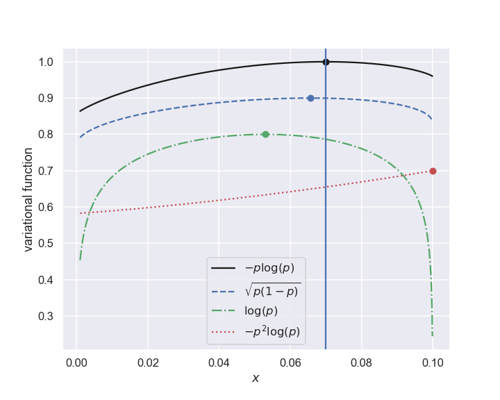
../../../_images/scandinavian_entropy.png — Fig. 12.2 Four different variational functions \(f\left( \{ p_i \} \right)\). The optimal \(x\) for each one is shown by a circle. The uncorrelated assignment \(x=0.07\) is shown by a vertical line.#

Continuous case#

Let us return to the monkeys, but now with different probabilities for each bin. Then

(12.17)#\[\begin{equation} S= −\sum_{i=1}^M p_i \log \left( \frac{p_i}{m_i} \right), \end{equation}\]

which is often known as the Shannon-Jaynes entropy, or the Kullback number, or the cross entropy (with opposite sign).

Jaynes (1963) has pointed out that this generalization of the entropy, including a Lebesgue measure \(m_i\), is necessary when we consider the limit of continuous parameters.

(12.18)#\[\begin{equation} S[p]= −\int p(x) \log \left( \frac{p(x)}{m(x)} \right). \end{equation}\]

In particular, \(m(x)\) ensures that the entropy expression is invariant under a change of variables \(x \to y=f(x)\).
Typically, the transformation-group (invariance) arguments are appropriate for assigning \(m(x) = \mathrm{constant}\).
However, there are situations where other assignments for \(m\) represent the most ignorance. For example, in counting experiments one might assign \(m(N) = M^N / N!\) for the number of observed events \(N\) and a very large number of intervals \(M\).

Derivation of common pdfs using MaxEnt#

The principle of maximum entropy (MaxEnt) allows incorporation of further information, e.g. constraints on the mean, variance, etc, into the assignment of probability distributions.

In summary, the MaxEnt approach aims to maximize the Shannon-Jaynes entropy and generates smooth functions.

Mean and the Exponential pdf#

Suppose that we have a pdf \(p(x|I)\) that is normalized over some interval \([ x_\mathrm{min}, x_\mathrm{max}]\). Assume that we have information about its mean value, i.e.,

(12.19)#\[\begin{equation} \langle x \rangle = \int x p(x|I) dx = \mu. \end{equation}\]

Based only on this information, what functional form should we assign for the pdf that we will now denote \(p(x|\mu)\)?

Let us use the principle of MaxEnt and maximize the entropy under the normalization and mean constraints. We will use Lagrange multipliers, and we will perform the optimization as a limiting case of a discrete problem; explicitly, we will maximize

(12.20)#\[\begin{equation} Q = -\sum_i p_i \log \left( \frac{p_i}{m_i} \right) + \lambda_0 \left( 1 - \sum_i p_i \right) + \lambda_1 \left( \mu - \sum_i x_i p_i \right). \end{equation}\]

Setting \(\partial Q / \partial p_j = 0\) we obtain

(12.21)#\[\begin{equation} p_j = m_j \exp \left[ -(1+\lambda_0) \right] \exp \left[ -\lambda_1 x_j \right]. \end{equation}\]

With a uniform measure \(m_j = \mathrm{constant}\) we find (in the continuous limit) that

(12.22)#\[\begin{equation} p(x|\mu) = \mathcal{N} \exp \left[ -\lambda_1 x \right]. \end{equation}\]

The normalization constant (related to \(\lambda_0\)) and the remaining Lagrange multiplier, \(\lambda_1\), can easily determined by fulfilling the two constraints.

Assuming, e.g., that the normalization interval is \(x \in [0, \infty[\) we obtain

(12.23)#\[\begin{equation} \int_0^\infty p(x|\mu) dx = 1 = \left[ -\frac{\mathcal{N}}{\lambda_1} e^{-\lambda_1 x} \right]_0^\infty = \frac{\mathcal{N}}{\lambda_1} \quad \Rightarrow \quad \mathcal{N} = \lambda_1. \end{equation}\]

The constraint for the mean then gives

(12.24)#\[\begin{equation} \mu = \lambda_1 \int_0^\infty x e^{-\lambda_1 x} dx = \lambda_1 \frac{1!}{\lambda_1^2} = \frac{1}{\lambda_1} \quad \Rightarrow \quad \lambda_1 = \frac{1}{\mu}. \end{equation}\]

So that the properly normalized pdf from MaxEnt principles becomes the exponential distribution

(12.25)#\[\begin{equation} p(x|\mu) = \frac{1}{\mu} \exp \left[ -\frac{x}{\mu} \right]. \end{equation}\]

Variance and the Gaussian pdf#

Suppose that we have information not only on the mean \(\mu\) but also on the variance

(12.26)#\[\begin{equation} \left\langle (x-\mu)^2 \right\rangle = \int (x-\mu)^2 p(x|I) dx = \sigma^2. \end{equation}\]

The principle of MaxEnt will then result in the continuum assignment

(12.27)#\[\begin{equation} p(x|\mu,\sigma) \propto \exp \left[ - \lambda_1 ( x - \mu )^2 \right]. \end{equation}\]

Assuming that the limits of integration are \(\pm \infty\) we can determine both the normalization coefficient and the Lagrange multiplier. After some integration this results in the standard Gaussian pdf

(12.28)#\[\begin{equation} p(x|\mu,\sigma) = \frac{1}{\sigma \sqrt{2\pi}} \exp \left[ - \frac{( x - \mu )^2}{2\sigma^2} \right]. \end{equation}\]

The normal distribution

This indicates that the normal distribution is the most honest representation of our state of knowledge when we only have information about the mean and the variance.

Notice. These arguments extend easily to the case of several parameters. For example, considering \(\{x_k\}\) as the data \(\{ D_k\}\) with error bars \(\{\sigma_k\}\) and \(\{\mu_k\}\) as the model predictions, this allows us to identify the least-squares likelihood as the pdf which best represents our state of knowledge given only the value of the expected squared-deviation between our predictions and the data

(12.29)#\[\begin{equation} p\left( \{x_k\} | \{\mu_k, \sigma_k\} \right) = \prod_{k=1}^N \frac{1}{\sigma_k \sqrt{2\pi}} \exp \left[ - \frac{( x_k - \mu_k )^2}{2\sigma_k^2} \right]. \end{equation}\]

If we had convincing information about the covariance \(\left\langle \left( x_i - \mu_i \right) \left( x_j - \mu_j \right) \right\rangle\), where \(i \neq j\), then MaxEnt would assign a correlated, multivariate Gaussian pdf for \(p\left( \{ x_k \} | I \right)\).

Poisson distribution#

The constraints are normalization and a known mean:

\[\begin{split}\begin{align} \int_{0}^\infty dx\, p(x) &= 1, \quad x\geq 0 \\ \int_{0}^\infty dx\, x p(x) &= \mu \end{align}\end{split}\]

\(\Lra\) maximize

\[ Q(p;\lambda_0,\lambda_1) = - \int dx\, p(x)\log\Bigl(\frac{p(x)}{m(x)}\Bigr) + \lambda_0 \bigl(1 - \int dx\, p(x)\bigr) + \lambda_1 \bigl(\mu - \int dx\, x p(x)\bigr) , \]

with uniform \(m(x)\). The maximization is again straightforward:

\[\begin{split}\begin{align} & \frac{\delta Q}{\delta p(x)} = -\log\frac{p(x)}{1} - \frac{p(x)}{p(x)} - \lambda_0 - \lambda_1 x = 0 \\ & \Lra \log p(x) = -(1 + \lambda_0) - \lambda_1 x \\ & \Lra p(x) = e^{-1+\lambda_0}e^{-\lambda_1 x} \end{align}\end{split}\]

Finally, we determine \(\lambda_0\) and \(\lambda_1\) from the constraints:

\[\begin{split}\begin{align} e^{1+\lambda_0}\int_0^\infty dx\, e^{-\lambda_1 x} = e^{-(1+\lambda_0)}\frac{1}{\lambda_1} = 1 \quad&\Lra\quad \lambda_1 = e^{-(1+\lambda_0)} \\ \int_0^\infty dx\, \underbrace{e^{-(1+\lambda_0)}}_{\lambda_1} \underbrace{e^{-\lambda_1 x}x}_{1/\lambda_1^2} = \mu \quad&\Lra\quad \lambda_1 = \frac{1}{\mu} . \end{align}\end{split}\]

Substituting we get the Poisson distribution:

\[ p(x) = \frac{1}{\mu} e^{-x/\mu} . \]

Log normal distribution#

Suppose the constraint is on the variance of \(\ln x\), i.e.,

\[ \int p(x)\left[\log\left(\frac{x}{x_0}\right)\right]^2 dx=\sigma^2 \]

Change variables to \(y=\log(x/x_0)\). What is the constraint in terms of \(y\)?

Now maximize the entropy, subject to this constraint, and, of course, the normalization constraint.

You should obtain the log-normal distribution:

\[ p(x)=\frac{1}{\sqrt{2 \pi} x \sigma} \exp\left[-\frac{\ln^2(x/x_0)}{2 \sigma^2}\right]. \]

When do you think it would make sense to say that we know the variance of \(\log(x)\), rather than the variance of \(x\) itself?

l1-norm#

Finally, we take the constraint on the mean absolute value of \(x-\mu\): \(\langle |x-\mu| \rangle=\epsilon\).

This constraint is written as:

\[ \int p(x) \, |x - \mu| \, dx=\epsilon. \]

Use the uniform measure, and go through the steps once again, to show that:

\[ p(x)=\frac{1}{2 \epsilon} \exp\left(-\frac{|x-\mu|}{\epsilon}\right). \]

Try other examples!