20.2. Sampling / Importance Resampling

Note

This chapter is reproduced (with some adjustments) from Bayesian probability updates using sampling/importance resampling: Applications in nuclear theory by Weiguang Jiang and Christian Forssén in Front. in Phys., 10:1058809, 2022 [JForssen22] (with permission).

The use of MCMC in the statistical analysis of complex computer models typically requires massive computations. There are certainly situations where MCMC sampling is not ideal, or even becomes infeasible:

1. When the posterior is conditioned on some calibration data for which the model evaluations are very costly. Then a limited number of full likelihood evaluations can be afforded and the MCMC sampling becomes less likely to converge.

2. Bayesian posterior updates in which calibration data is added in several different stages. This typically requires that the MCMC sampling must be carried out repeatedly from scratch.

3. Model checking where the sensitivity to prior assignments is being explored. This is a second example of posterior updating.

4. The prediction of target observables for which model evaluations become very costly and the handling of a large number of MCMC samples becomes infeasible.

These are situations where one might want to use the Sampling/Importance Resampling (S/IR) method [BS06, SG92], which can exploit the previous results of model evaluations to allow posterior probability updates at a much smaller computational cost compared to the full MCMC method.

Brief review of the method

The basic idea of S/IR is to utilize the inherent duality between samples and the density (probability distribution) from which they were generated [SG92]. This duality offers an opportunity to indirectly recreate a density (that might be hard to compute) from samples that are easy to obtain.

Let us consider a target density \(h(\pars)\). This could be a posterior PDF \(\pdf{\pars}{\data, I}\). Instead of attempting to directly collect samples from \(h(\pars)\), as would be the goal in MCMC approaches, the S/IR method uses a detour. We first obtain samples from a simple (even analytic) density \(g(\pars)\). We then resample from this finite set using a resampling algorithm to approximately recreate samples from the target density \(h(\pars)\). There are (at least) two different resampling methods. In this paper we only focus on one of them called weighted bootstrap (more details of resampling methods can be found in Refs. [Rub88, SG92]).

Assuming we are interested in the target density \(h(\pars)=f(\pars)\,/\int\! f(\pars)\,\mathrm{d}\pars\), the procedure of resampling via weighted bootstrap can be summarized as follows:

Algorithm 20.2 (The Sampling/Importance Resampling method)

1. Generate the set \(\{ \pars_i\}_{i=1}^n\) of samples from a sampling density \(g(\pars)\).

2. Calculate \(\omega_i=f(\pars_i)\,/\,g(\pars_i)\) for the \(n\) samples and define importance weights as: \(q_i=\omega_i~/\sum_{j=1}^n \omega_j\).

3. Draw \(N\) new samples \(\{ \optpars_i\}_{i=1}^N\) from the discrete distribution \(\{ \pars_i \}_{i=1}^n\) with probability mass \(q_i\) on \(\pars_i\).

4. The set of samples \(\{ \optpars_i \}_{i=1}^N \) will then be approximately distributed according to the target density \(h(\pars)\).

Intuitively, the distribution of \(\optpars\) should be good approximation of \(h(\pars)\) when \(n\) is large enough. Here we justify this claim via the cumulative distribution function of \(\optpara\) (for the one-dimensional case)

(20.6)\[\begin{split} \begin{aligned} \rm{pr}(\optpara\leq a) &= \sum\limits_{i=1}^n q_i \cdot H(a-\para_i) = \frac{ \frac{1}{n}\sum\limits_{i=1}^n \omega_i \cdot H(a-\para_i)}{ \frac{1}{n}\sum\limits_{i=1}^n \omega_i} \\ & \xrightarrow[n \rightarrow \infty]{} \frac{\mathbb{E}_g\left[ \frac{f(\para)}{g(\para)} \cdot H(a-\para) \right]}{\mathbb{E}_g\left[\frac{f(\para)}{g(\para)}\right]} = \frac{\int^{a}_{-\infty}f(\para)\,d\para}{\int^{\infty}_{-\infty}f(\para)\,d\para}= \int^{a}_{-\infty}h(\para)\,d\para , \end{aligned} \end{split}\]

with \(\mathbb{E}_g[X(\para)]=\int^{\infty}_{-\infty} X(\para) g(\para)\,d\para\) the expectation value of \(X(\para)\) with respect to \(g(\para)\), and \(H\) Heaviside step function such that

(20.7)\[\begin{split} H(a-\para) = \begin{cases} 1 & \text{if}\ \para \leq a, \\ 0 & \text{if}\ \para > a . \end{cases} \end{split}\]

The above resampling method can be applied to generate samples from the posterior PDF \(h(\pars)=\rm{pr}(\pars|\mathcal{D})\) in a Bayesian analysis. It remains to choose a sampling distribution, \(g(\pars)\), which in principle could be any continuous density distribution. However, recall that \(h(\pars)\) can be expressed in terms of an unnormalized distribution \(f(\pars)\), and using Bayes’ theorem we can set \(f(\pars)=\mathcal{L}(\pars)\pdf{\pars}{I}\). Thus, choosing the prior \(\pdf{\pars}{I}\) as the sampling distribution \(g(\pars)\) we find that the importance weights are expressed in terms of the likelihood, \(q_i = \mathcal{L}(\pars_i)/ \sum_{j=1}^n \mathcal{L}(\pars_j)\). Assuming that it is simple to collect samples from the prior, the costly operation will be the evaluation of \(\mathcal{L}(\pars_i)\). Here we make the side remark that an effective and computationally cost-saving approximation can be made if we manage to perform a pre-screening to identify (and ignore) samples that will give a very small importance weight. We also note that the above choice of \(g(\pars)=\rm{pr}(\pars)\) is purely for simplicity and one can perform importance resampling with any \(g(\pars)\).

Example 20.1 (Illustration of S/IR)

Let us follow the above procedure in a simple example of S/IR to illustrate how to get samples from a posterior distribution. We consider a two-dimensional parametric model with \(\pars = (\para_1\), \(\para_2)\). Given data \(\mathcal{D}\) obtained under the model we have:

(20.8)\[ \pdf{\para_1,\para_2}{\data} = \frac{ \mathcal{L}(\para_1,\para_2)\pdf{\para_1,\para_2}{I}}{\iint \mathcal{L}(\para_1,\para_2) \pdf{\para_1,\para_2}{I} \, d\para_1 d\para_2}. \]

For simplicity and illustration, the joint prior distribution for \(\para_1\), \(\para_2\) is set to be uniform over the unit square as shown in Fig. 20.1a. In this example we also assume that the data \(\data\) likelihood is described by a multivariate Student-t distribution

(20.9)\[ \mathcal{L}(\para_1,\para_2) = \frac{\Gamma[(\nu+p)/2]}{\Gamma(\nu/2)\nu^{p/2}\pi^{p/2}|\boldsymbol{\Sigma}|^{1/2}}\left[ {1+\frac{1}{\nu}(\pars-\boldsymbol{\mu})^{T}\boldsymbol{\Sigma}^{-1}(\pars-\boldsymbol{\mu})} \right]^{-(\mu+p)/2}, \]

where the dimension \(p=2\), the degrees of freedom \(\nu=2\), the mean vector \(\boldsymbol{\mu} = (0.2, 0.5)\) and the scale matrix \(\boldsymbol\Sigma=[[0.02, 0.005], [0.005, 0.02]]\).

The importance weights \(q_i\) are then computed for \(n=2000\) samples drawn from the prior (these prior samples are shown in Fig. 20.1a). The resulting histogram of importance weights is shown in Fig. 20.1b. Here the weights have been rescaled as \(\tilde{q}_i=q_i/\max(\{ q \})\) such that the sample with the largest probability mass corresponds to 1 in the histogram. We also define the effective number of samples, \(n_\mathrm{eff}\), as the sum of rescaled importance weights, \(n_\mathrm{eff} = \sum_{i=1}^n \tilde{q}_i\). Finally, in Fig. 20.1c we show \(N=20,000\) new samples \(\{ \optpars_i \}_{i=1}^N\) that are drawn from the prior samples \(\{ \pars_i\}_{i=1}^n\) according to the probability mass \(q_i\) for each \(\pars_i\). The blue and green contour lines represent (68% and 90%) credible regions for the resampled distribution and for the Student-t distribution, respectively. This result demonstrates that the samples generated by the S/IR method give a very good approximation of the target posterior distribution.

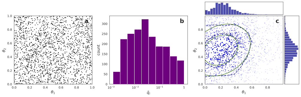
Fig. 20.1 Illustration of S/IR procedures. a. Samples \(\{ \pars\}_{i=1}^n\) from a uniform prior in a unit square (\(n=2000\) samples are shown). b. Histogram of rescaled importance weights \(\tilde{q}_i=q_i/\max(\{q\})\) where \(q_i= \mathcal{L}(\pars_i)/ \sum_{j=1}^n \mathcal{L}(\pars_j)\) with \(\mathcal{L}(\pars)\) as in Eq. (20.9). The number of effective samples is \(n_\mathrm{eff}=214.6\). Note that the samples are drawn from a unit square and that the tail of the target distribution is not covered. c. Samples \(\{ \optpars\}_{i=1}^N\) of the posterior (blue dots with 10% opacity) resampled from the prior samples with probability mass \(q_i\). The contour lines for the \(68\%\) and \(90\%\) credible regions of the posterior samples (blue dashed) are shown and compared with those of the exact bivariate target distribution (green solid). Summary histograms of the marginal distributions for \(\para_1\) and \(\para_2\) are shown in the top and right subplots.

S/IR limitations

While the S/IR approach might provide a useful alternative to full MCMC sampling, there are some important limitations. In particular, users should be mindful of the effective number of samples. The more complex the likelihood function, the less effective is the use of a sampling distribution.

Unfortunately one can also envision more difficult scenarios in which S/IR could fail without any clear signatures. For example, if the prior has a very small overlap with the posterior there is a risk that many prior samples get a similar importance weight (such that the number of effective samples is large) but that one has missed the most interesting region. Prior knowledge of the posterior landscape is very useful to avoid possible failure scenarios that might not be signaled by the number of effective samples.