Overview of diagnostics for MCMC sampling

19.2. Overview of diagnostics for MCMC sampling#

We’ve seen that using MCMC with the Metropolis-Hastings algorithm (or an alternative algorithm) leads to a Markov chain: a set of configurations of the parameters we are sampling. This chain enables inference because they are samples of the posterior of interest. MCMC sampling is notoriously difficult to validate. In this section we will discuss some common convergence tests.

Convergence tests for MCMC sampling#

MCMC sampling can go wrong in (at least) three ways:

No convergence—The limiting distribution is not reached.
Pseudoconvergence—The chain seems stationary, but the limiting distribution is not actually reached.
Highly correlated samples—Not really wrong, but inefficient.

There is no unique solution to such problems, but they are typically addressed in three ways:

Design the simulation runs for monitoring of convergence. In particular, run multiple sequences of the Markov chains with starting points dispersed over the sampling space. This is difficult in high dimensions.
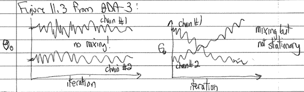
Monitor the convergence of individual sampling dimensions, as well as predicted quantities of interest, by comparing variations within and between the different sequences (chains). Here you are looking for stationarity (the running means are stable) and mixing (different sequences are sampling the same distribution). The Gelman-Rubin test (see below) is devised for this purpose. In the following schematic version of Figure 11.3 in BDA-3, we see on the left two chains that stay in separate regions of \(\theta_0\) (no mixing) while on the right there is mixing but neither chain shows a stationary distribution (the \(\theta_0\) distribution keeps changing with MC steps).

Unacceptably inefficient sampling (too low acceptance rate) implies that the algorithm must be adjusted, or that an altogether different sampling algorithm should be used.

The diagnostics that will be discussed below are all univariate. They work perfectly when there is only one parameter to estimate. In fact, most convergence tests are performed with univariate diagnostics applied to each sampling dimension one by one.

Variance of the mean#

Consider the sampling variance of a parameter mean value

(19.1)#\[ \var{\bar\para} = \frac{\var{\para}}{N}, \]

where \(N\) is the length of the chain. This quantity is capturing the simulation error of the mean rather than the underlying uncertainty of the parameter \(\para\). We can visualize this by examining the moving average of our parameter trace. The trace is the sequence as a function of iteration number.

Autocorrelation#

A challenge when doing MCMC sampling is that the collected samples can be correlated. This can be tested by computing the autocorrelation function and extracting the correlation time for a chain of samples.

Say that \(X\) is an array of \(N\) samples numbered by the index \(t\). Then \(X_{+h}\) is a shifted version of \(X\) with elements \(X_{t+h}\). The integer \(h\) is called the lag. Since we have a finite number of samples, the array \(X_{+h}\) will be \(h\) elements shorter than \(X\).

Furthermore, \(\bar{X}\) is the average value of \(X\).

We can then define the autocorrelation function \(\rho(h)\) from the list of samples.

(19.2)#\[ \rho(h) = \frac{\sum_{t=0}^{N-h-1} \left[ (X_t - \bar{X}) (X_{t+h} - \bar{X})\right]} {\sqrt{ \sum_{t=0}^{N-h-1} (X_t - \bar{X})^2 } \sqrt{ \sum_{t=0}^{N-h-1} (X_{t+h} - \bar{X})^2 }} \]

The summation is carried out over the subset of samples that overlap. The autocorrelation is the overlap (scalar product) of the chain of samples (the trace) with a copy of itself shifted by the lag, as a function of the lag. If the lag is short so that nearby samples are close to each other (and have not moved very far) the product of these two vectors is large. If samples are independent, you will have both positive and negative numbers in the overlap that cancel each other.

The typical example of a highly correlated chain is a random walk with a too short proposal step length.

It is often observed that \(\rho(h)\) is roughly exponential so that we can define an autocorrelation time \(\tau_\mathrm{a}\) according to \(\rho(h) \sim \exp(-h/\tau_\mathrm{a})\).

The integrated autocorrelation time is

\[ \tau = 1 + 2 \lim_{N \to \infty} \sum_{h=1}^N \rho(h). \]

With autocorrelated samples, the sampling variance (19.1) becomes

(19.3)#\[ \var{\bar\para} = \tau \frac{\var{\para}}{N}, \]

with \(\tau \gg 1\) for highly correlated samples. This motivates us to define the effective sample size (ESS) as

\[ \text{ESS} = N / \tau. \]

To keep ESS high, we must collect many samples and keep the autocorrelation time small.

The Gelman-Rubin test#

The Gelman-Rubin diagnostic was constructed to test for stationarity and mixing of different Markov chain sequences [GR92].

Algorithm 19.1 (The Gelman-Rubin diagnostic)

Collect \(M>1\) sequences (chains) of length \(2N\).
Discard the first \(N\) draws of each sequence, leaving the last \(N\) iterations in the chain.
Calculate the within and between chain variance.
- Within chain variance:
  
  \[ W = \frac{1}{M}\sum_{j=1}^M s_j^2 \]
  
  where \(s_j^2\) is the variance of each chain (after throwing out the first \(N\) draws).
- Between chain variance:
  
  \[ B = \frac{N}{M-1} \sum_{j=1}^M (\bar{\para} - \bar{\bar{\para}})^2 \]
where \(\bar{\bar{\para}}\) is the mean of each of the M means.
Calculate the estimated variance of \(\theta\) as the weighted sum of between and within chain variance.

\[ \widehat{\var{\para}} = \left ( 1 - \frac{1}{N}\right ) W + \frac{1}{N}B \]

Calculate the potential scale reduction factor.

\[ \hat{R} = \sqrt{\frac{\widehat{\var{\para}}}{W}} \]

We want the \(\hat{R}\) number to be close to 1 since this would indicate that the between chain variance is small. And a small chain variance means that both chains are mixing around the stationary distribution. Gelman and Rubin [GR92] showed that stationarity has certainly not been achieved when \(\hat{R}\) is greater than 1.1 or 1.2.