27. Bayesian neural networks#
The introduction part of this lecture is inspired by the chapter “Learning as Inference” in the excellent book Information Theory, Inference, and Learning Algorithms by David MacKay [Mac03].
Some python libraries that are relevant for Bayesian Neural Networks (and part of the general trend towards Probabilistic Programming in Machine Learning) are:
Keras (for constructing tensorflow models).
27.1. Basic neural network#
We will consider a neuron with a vector of \(I\) input signals \(\boldsymbol{x} = \left\{ \boldsymbol{x}^{(i)} \right\}_{i=1}^I\), and an output signal \(y^{(i)}\), which is given by the non-linear function \(y(z)\) of the activation
where \(\boldsymbol{w} = \left\{ w_i \right\}_{i=1}^I\) are the weights of the neuron and we have included a bias (\(b \equiv w_0\)).
The training of the network implies feeding it with training data and finding the sets of weights and biases that minimizes a loss function that has been selected for that particular problem. Consider, e.g., a classification problem where the single output \(y\) of the final network layer is a real number \(\in [0,1]\) that indicates the (discrete) probability for input \(\boldsymbol{x}\) belonging to either class \(t=1\) or \(t=0\):
A simple binary classifier can be trained by minimizing the loss function
made up of an error function
where \(t^{(n)}\) is the training data, and the regularizer
that is designed to avoid overfitting. The error function can be interpreted as minus the log likelihood, with the likelihood
Similarly the regularizer can be interpreted in terms of a log prior probability distribution over the parameters. With the quadratic \(E_W\) given above, the corresponding prior distribution is a Gaussian with variance \(\sigma_W^2 = 1/\alpha\) and \(1/Z_W = (\alpha/2\pi)^{K/2}\), where \(K\) is the number of parameters in \(w\).
The objective function \(C_W(w)\) then corresponds to the inference of the parameters \(\boldsymbol{w}\) given the data
We show the evolution of the probability distribution for a sequence of an increasing number of training data (\(N\)) in Fig. 27.1. The targets are either 0 or 1, as indicated by red and blue markers. The network parameters \(\boldsymbol{w}\) that are found by minimizing \(C_W(\boldsymbol{w})\) can be interpreted as the most probable parameter vector \(\boldsymbol{w}^*\).
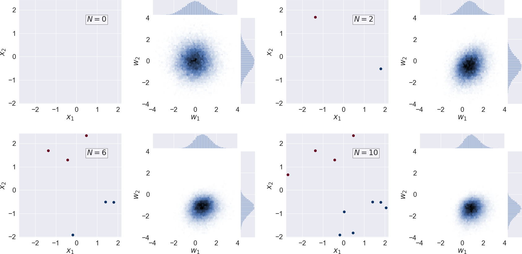
Fig. 27.1 Scatter plot of training data and the corresponding bivariate posterior pdf for the neuron weights \(p(w_1, w_2 | \mathcal{D}, \alpha)\) (i.e. marginalized over the bias \(w_0\)) for a sequence of \(N=0,2,6,10\) training data.#
In the following, we will rather use the Bayesian approach and consider the information that is contained in the actual probability distribution. In fact, there are different uncertainties that should be addressed:
Epistemic uncertainties
correspond to uncertainties in the model. For a neural network we can learn about this uncertainty using test data. Epistemic uncertainty is also known as systematic uncertainty.
Aleatoric uncertainties
appear as a result of inherent noise in the training data. This should be included in the likelihood function (and is therefore part of the Bayesian approach). It can, however, not be reduced with more data of the same quality. Aleatoric uncertainty is also known as statistical uncertainty. Aleatoric is derived from the Latin alea or dice, referring to a game of chance.
Notice. We will use \(y\) to denote the output from the neural network. For classification problems, \(y\) will give the categorical (discrete) distribution of probabilities \(p_{t=c}\) of belonging to class \(c\). For regression problems, \(y\) is a continuous variable. It could also, in general, be a vector of outputs. The neural network can be seen as a non-linear mapping \(y(x; w)\): \(x \in \mathbb{R}^p \to y \in \mathbb{R}^m\).
27.2. Probabilistic model#
A Bayesian neural network can be viewed as probabilistic model in which we want to infer \(p(y \lvert \boldsymbol{x},\mathcal{D})\) where \(\mathcal{D} = \left\{\boldsymbol{x}^{(i)}, y^{(i)}\right\}\) is a given training dataset.
We construct the likelihood function \(p(\mathcal{D} \lvert \boldsymbol{w}) = \prod_i p(y^{(i)} \lvert \boldsymbol{x}^{(i)}, \boldsymbol{w})\) which is a function of parameters \(\boldsymbol{w}\). Maximizing the likelihood function gives the maximimum likelihood estimate (MLE) of \(\boldsymbol{w}\). The usual optimization objective during training is the negative log likelihood. For a categorical distribution this is the cross entropy error function, for a Gaussian distribution this is proportional to the sum of squares error function. MLE can lead to severe overfitting though.
Multiplying the likelihood with a prior distribution \(p(\boldsymbol{w})\) is, by Bayes theorem, proportional to the posterior distribution \(p(\boldsymbol{w} \lvert \mathcal{D}) \propto p(\mathcal{D} \lvert \boldsymbol{w}) p(\boldsymbol{w})\). Maximizing \(p(\mathcal{D} \lvert \boldsymbol{w}) p(\boldsymbol{w})\) gives the maximum a posteriori (MAP) estimate of \(\boldsymbol{w}\). Computing the MAP estimate has a regularizing effect and can prevent overfitting. The optimization objectives here are the same as for MLE plus a regularization term coming from the log prior.
Both MLE and MAP give point estimates of parameters. If we instead had a full posterior distribution over parameters we could make predictions that take weight uncertainty into account. This is covered by the posterior predictive distribution \(p(y \lvert \boldsymbol{x},\mathcal{D}) = \int p(y \lvert \boldsymbol{x}, \boldsymbol{w}) p(\boldsymbol{w} \lvert \mathcal{D}) d\boldsymbol{w}\) in which the parameters have been marginalized out. This is equivalent to averaging predictions from an ensemble of neural networks weighted by the posterior probabilities of their parameters \(\boldsymbol{w}\).
Returning to the binary classification problem, \(y^{(n+1)}\) corresponds to the probability \(p_{t^{(n+1)}=1}\) and a Bayesian prediction of a new datum \(y^{(n+1)}\) will correspond to a pdf and involves marginalizing over the weight and bias parameters
where we have also included the weight decay hyperparameter \(\alpha\) from the prior (regularizer). Marginalization could, of course, also be performed over this parameter.
We show an example of such inference, comparing the point estimate \(y(x; w^*, \alpha)\) and the Bayesian approach, in Fig. 27.2.
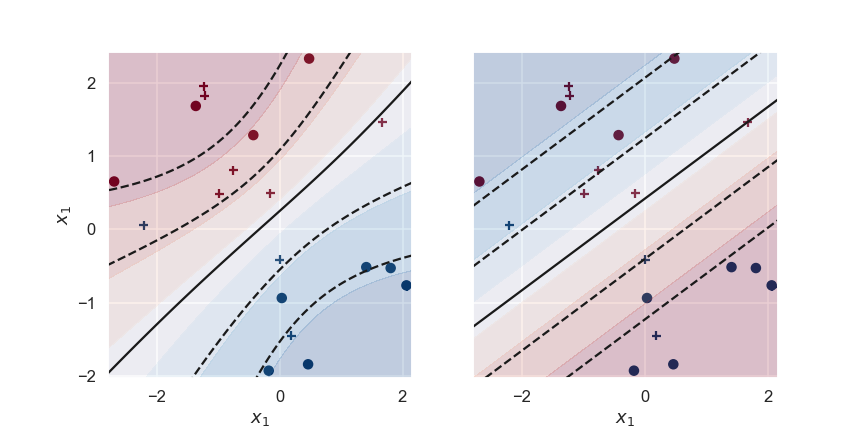
Fig. 27.2 The predictions for a Bayesian (left panel) and regular (right panel) binary classifier that has been learning from ten training data (circles) with a weight decay \(\alpha = 1.0\). The decision boundary (\(y=0.5\), i.e. the activation \(a=0\)) is shown together with the levels 0.12,0.27,0.73,0.88 (corresponding to the activation \(a=\pm1,\pm2\)). Test data is shown as plus symbols.#
The Bayesian classifier is based on sampling a very large ensamble of single neurons with different parameters. The distribution of these samples will be proportional to the posterior pdf for the parameters. The decision boundary shown in the figure is obtained as the mean of the predictions of the sampled neurons evaluated on a grid. It is clear that the Bayesian classifier is more uncertain about its predictions in the lower left and upper right corners, where there is little training data.
This becomes even more clear when we plot the standard deviation of the predictions of the Bayesian classifier in Fig. 27.3.
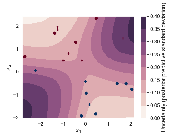
Fig. 27.3 The standard deviation of the class label predictions for a Bayesian binary classifier.#
The predictions are rather certain along a diagonal line (close to the training data). Note that the interpretation of the prediction in the center of Fig. 27.3 (near \(x_1,x_2 = 0,0\)) is the following: The Bayesian binary classifier predicts a probability of \(\sim 0.5\) for this point in the input parameter space to belong to class 1 (i.e. the decision is very uncertain). The Baysian classifier is also very certain about this uncertainty (the standard deviation is small).
In contrast, predictions for points in the upper left or lower right corners are very certain about the class label (and there is little uncertainty about this certainty).
27.3. Bayesian neural networks in practice#
How can we compute the marginalization integral for neural networks with thousands of parameters?
In short, there are three different approaches:
Sampling methods, e.g. MCMC (this approach would be exact as the number of samples \(\rightarrow \infty\));
Deterministic approximate methods, for example using Gaussian approximations with the Laplace method;
Variational methods.
The first two have been discussed previously in these notes in the general context of Bayesian inference. In the following, we will focus on the variational methods.
Variational inference for Bayesian neural networks#
Bayesian neural networks differ from plain neural networks in that their weights are assigned a probability distribution instead of a single value or point estimate. These probability distributions describe the uncertainty in weights and can be used to estimate uncertainty in predictions.
Unfortunately, full inference of the weight posterior \(p(\boldsymbol{w} \lvert \mathcal{D})\) for neural networks is usually intractable due to the large dimensionality. Instead we can attempt to approximate the true posterior with a proxy distribution \(q(\boldsymbol{w} \lvert \boldsymbol{\theta})\) with variational parameters that we want to estimate.
Training a Bayesian neural network via variational inference implies learning the parameters of the proxy distribution rather than learning the real posterior.
This can be done by minimizing the Kullback-Leibler divergence between \(q(\boldsymbol{w} \lvert \boldsymbol{\theta})\) and the true posterior \(p(\boldsymbol{w} \lvert \mathcal{D})\) w.r.t. \(\boldsymbol{\theta}\).
The specific goal is then to replace \(p(\boldsymbol{w} \lvert \mathcal{D})\), which we don’t know, with the known proxy distribution \(q(\boldsymbol{w} \lvert \boldsymbol{\theta}^*)\), where \(\boldsymbol{\theta}^*\) is the optimal set of variational parameters.
The Kullback-Leibler divergence#
The KL divergence is a numeric measure of the difference between two distributions. For two probability distributions \(q(\boldsymbol{w})\) and \(p(\boldsymbol{w})\), the KL divergence in a continuous case,
As we can see, the KL divergence corresponds to the expected log difference between two distributions with respect to distribution \(q\). It is a non-negative quantity and it is equal to zero only when the two distributions are identical.
Intuitively there are three scenarios:
if both \(q\) and \(p\) are high at the same positions, then we are succeeding;
if \(q\) is high where \(p\) is low, we pay a price;
if \(q\) is low we don’t care about \(p\) (because of the expectation).
The divergence measure is not symmetric, i.e., \(D_\mathrm{KL}(p||q) \neq D_\mathrm{KL}(q||p)\). In fact, it is possibly more natural to reverse the arguments and compute \(D_\mathrm{KL}(p||q)\). However, we choose \(\mathrm{KL}(q||p)\) so that we can take expectations with respect to the known \(q(\boldsymbol{w})\) distribution. In addition, the minimization of this KL divergence will encourage the fit to concentrate on plausible parameters since
To minimize the first term we have to avoid putting probability mass into regions of implausible parameters. To minimize the second term we have to maximize the entropy of the variational distribution \(q\) as this term corresponds to its negative entropy.
Evidence Lower Bound#
Let us rewrite the posterior pdf \(p(\boldsymbol{w} \lvert \mathcal{D})\) using Bayes theorem
Note that the logarithm of the last term has no dependence on \(\boldsymbol{w}\) and the integration of \(q\) will just give one since it should be a properly normalized pdf. This term is then the log marginal likelihood (or model evidence). Furthermore, since the KL divergence on the left hand side is bounded from below by zero we get the Evidence Lower Bound (ELBO)
Variational inference was originally inspired by work in statistical physics, and with that analogy, \(-J_\mathrm{ELBO}(\boldsymbol{\theta})\) is also called the variational free energy and sometimes denoted \(\mathcal{F}(\mathcal{D},\boldsymbol{\theta})\).
The task at hand is therefore to find the set of parameters \(\boldsymbol{\theta}^*\) that maximizes \(J_\mathrm{ELBO}(\boldsymbol{\theta})\). The hardest term to evaluate is obviously the expectation of the log-likelihood
This problem constitutes a new and active area of research in machine learning and it permeates well with the overarching theme of this course. We will end by giving two pointers to further readings on this subject.
Bayesian neural networks in PyMC3#
In the demonstration notebook of this lecture, it is shown how to use Variational Inference in PyMC3 to fit a simple Bayesian Neural Network. That implementation is based on the Automatic Differentation Variational Inference (ADVI) approach, described e.g. in Automatic Variational Inference in Stan [KRGB15].
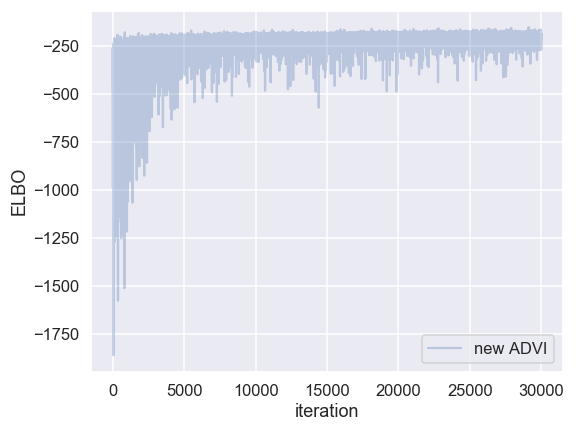
Fig. 27.4 The training of the Bayesian binary classifier, that employs ADVI implemented in pymc3, corresponds to modifying the variational distribution’s hyperparameters in order to maximize the Evidence Lower Bound (ELBO).#
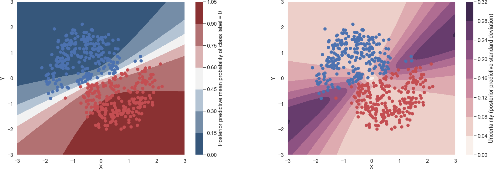
Fig. 27.5 The predictions for a Bayesian binary classifier that has been learning using ADVI implemented in pymc3. The mean (left panel) and standard deviation (right panel) of the binary classifier’s label predictions are shown.#
See also
Kucukelbir, A., Tran, D., Ranganath, R., Gelman, A., and Blei, D. M. (2016). Automatic Differentiation Variational Inference. arXiv: 1603.00788.
Bayes by Backprop#
The well-cited paper paper: Weight Uncertainty in Neural Networks (Bayes by Backprop) [BCKW15] has been well described in the blog entry by Martin Krasser. The main points of this blog entry are reproduced below with some modifications and some adjustments of notation.
All three terms in equation (27.12) are expectations w.r.t. the variational distribution \(q(\boldsymbol{w} \lvert \boldsymbol{\theta})\). In this paper they use the variational free energy \(\mathcal{F}(\mathcal{D},\boldsymbol{\theta}) \equiv -J_\mathrm{ELBO}(\boldsymbol{\theta})\) as a cost function (since it should be minimized). This quantity can be approximated by drawing Monte Carlo samples \(\boldsymbol{w}^{(i)}\) from \(q(\boldsymbol{w} \lvert \boldsymbol{\theta})\).
In the example used in the blog post, they use a Gaussian distribution for the variational posterior, parameterized by \(\boldsymbol{\theta} = (\boldsymbol{\mu}, \boldsymbol{\sigma})\) where \(\boldsymbol{\mu}\) is the mean vector of the distribution and \(\boldsymbol{\sigma}\) the standard deviation vector. The elements of \(\boldsymbol{\sigma}\) are the elements of a diagonal covariance matrix which means that weights are assumed to be uncorrelated. Instead of parameterizing the neural network with weights \(\boldsymbol{w}\) directly, it is parameterized with \(\boldsymbol{\mu}\) and \(\boldsymbol{\sigma}\) and therefore the number of parameters are doubled compared to a plain neural network.
Network training#
A training iteration consists of a forward-pass and and backward-pass. During a forward pass a single sample is drawn from the variational posterior distribution. It is used to evaluate the approximate cost function defined by equation (27.14). The first two terms of the cost function are data-independent and can be evaluated layer-wise, the last term is data-dependent and is evaluated at the end of the forward-pass. During a backward-pass, gradients of \(\boldsymbol{\mu}\) and \(\boldsymbol{\sigma}\) are calculated via backpropagation so that their values can be updated by an optimizer.
Since a forward pass involves a stochastic sampling step we have to apply the so-called re-parameterization trick for backpropagation to work. The trick is to sample from a parameter-free distribution and then transform the sampled \(\boldsymbol{\epsilon}\) with a deterministic function \(t(\boldsymbol{\mu}, \boldsymbol{\sigma}, \boldsymbol{\epsilon})\) for which a gradient can be defined. In the blog post they choose \(\boldsymbol{\epsilon}\) to be drawn from a standard normal distribution i.e. \(\boldsymbol{\epsilon} \sim \mathcal{N}(\boldsymbol{0}, \boldsymbol{I})\) and the function \(t\) is taken to be \(t(\boldsymbol{\mu}, \boldsymbol{\sigma}, \boldsymbol{\epsilon}) = \boldsymbol{\mu} + \boldsymbol{\sigma} \odot \boldsymbol{\epsilon}\), i.e., it shifts the sample by mean \(\boldsymbol{\mu}\) and scales it with \(\boldsymbol{\sigma}\) where \(\odot\) is element-wise multiplication.
For numerical stability the network is parametrized with \(\boldsymbol{\rho}\) instead of \(\boldsymbol{\sigma}\) and \(\boldsymbol{\rho}\) is transformed with the softplus function to obtain \(\boldsymbol{\sigma} = \log(1 + \exp(\boldsymbol{\rho}))\). This ensures that \(\boldsymbol{\sigma}\) is always positive. As prior, a scale mixture of two Gaussians is used \(p(\boldsymbol{w}) = \pi \mathcal{N}(\boldsymbol{w} \lvert 0,\sigma_1^2) + (1 - \pi) \mathcal{N}(\boldsymbol{w} \lvert 0,\sigma_2^2)\) where \(\sigma_1\), \(\sigma_2\) and \(\pi\) are shared parameters. Their values are learned during training (which is in contrast to the paper where a fixed prior is used).
See Martin Krasser’s blog entry for results and further details.