11.3. The ball-drop model

Sunil Jaiswal has developed a nice Jupyter notebook illustrating with the Ball Drop Experiment how the BOH approach works for robust extraction of physical quantities from a calibration. In the example one seeks a value for the acceleration due to gravity \(g\) using a theoretical model without air resistance fitted to data on height vs. time that includes air resistance and measurement errors. (A more general version with results shown below also has measurements of velocity and acceleration.) One first sees that a discrepancy model is essential; using a radial basis function (RBF) GP is standard (see Wikipedia RBF article) and one finds good predictions for times where there is data (this is KOH). But the discrepancy model must be more informed for a robust extraction of \(g\); this leads to using a nonstationary GP. Sunil has given permission for us to adapt his notebook. This example has many extensions available to students.

We test the model discrepancy framework on a simple system (popularized by statistician Dave Higdon) in which a ball is dropped from a tower of height \(h_0=60\,\)m at time \(t=0\,\)s. Measurements of the ball’s height above the ground, velocity, and acceleration are recorded at discrete time points until \(t=1\),s. (In this example \(x=t\)/(1,s) serves as the unitless input parameter, \(0\leq x \leq 1\).) The true theory, used to generate mock experimental data, incorporates a gravitational force \(\mathbf{f}_G=-Mg\,\hat{\bf z}\) and a drag force given by \(\mathbf{f}_D = -0.4 v^2\, \hat{\bf{v}}\). Here, \(M=1\,\)kg is the mass of the ball, \(g=9.8\,{\rm m/s}^2\) the acceleration due to gravity, and we set the initial velocity \(v_0\) to \(v_0=0\,\)m/s.

We assume that the observational errors for height, velocity, and acceleration are independent and identically distributed Gaussian random variables.

Mock experimental data are generated by sampling from Gaussian distributions with specified standard deviations and with means given by the predictions of the true theory, which are determined by the equations of motion: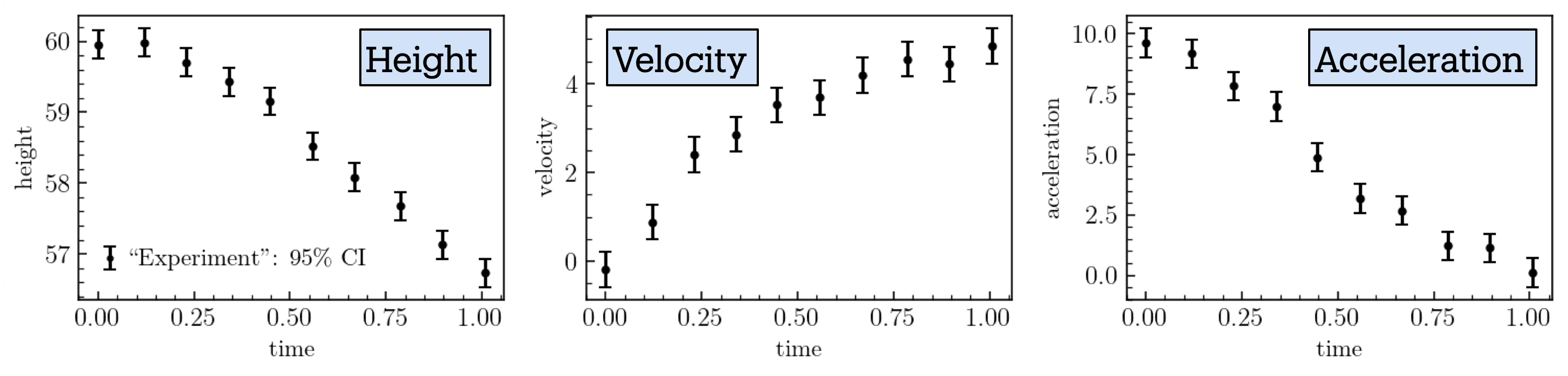

(11.6)\[ a = \frac{d v}{dt} = g - 0.4 v |v| \,, \qquad \frac{dh}{dt} = -v . \]

Fig. 11.3 Data for the ball drop experiment, including measurement errors.

We compare these mock data with a theoretical model that neglects the drag force and is governed by the simpler equations of motion:

\[ v = v_0 + g t \,, \qquad h = h_0 - v_0 t - \frac{1}{2} g t^2 . \]

Here \(h_0=60\,\)m is fixed to the value used in generating the mock experimental data. The parameters \(g\) and \(v_0\) are model parameters, which we infer using Bayesian parameter inference (in the notebook, for simplicity, only \(g\) is inferred). We incorporate our prior knowledge about the theory’s domain using the two distinct GP kernels discussed earlier. Since our model neglects drag forces, we are more confident in its predictions at earlier times (small \(x\)), when the velocity is lower, than at later times (larger \(x\)).

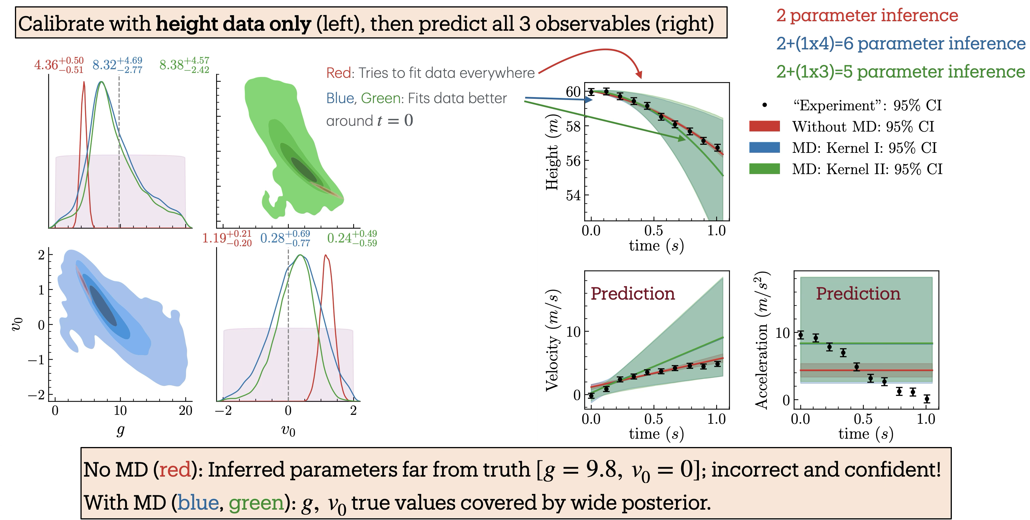
Fig. 11.4 Balldrop analysis with only the height measurements.

Fig. 11.4 shows both the inferred posteriors for the model parameters and the corresponding model predictions when only the height data is used. We perform Bayesian parameter inference under three scenarios: (i) without the model discrepancy (MD) term (red), (ii) with MD using GP-kernel \(\texttt{I}\) (blue), and (iii) with MD using GP-kernel \(\texttt{II}\) (green). The kernels are defined in Fig. 11.5; their hyperparameters are learned at the same time as the model parameters. Parameter inference is carried out by sequentially incorporating additional observables to examine their influence on the inferred posteriors. The posteriors and predictions for when height and velocity are included are shown in Fig. 11.6 and when height, velocity, and acceleration included are shown in Fig. 11.7.

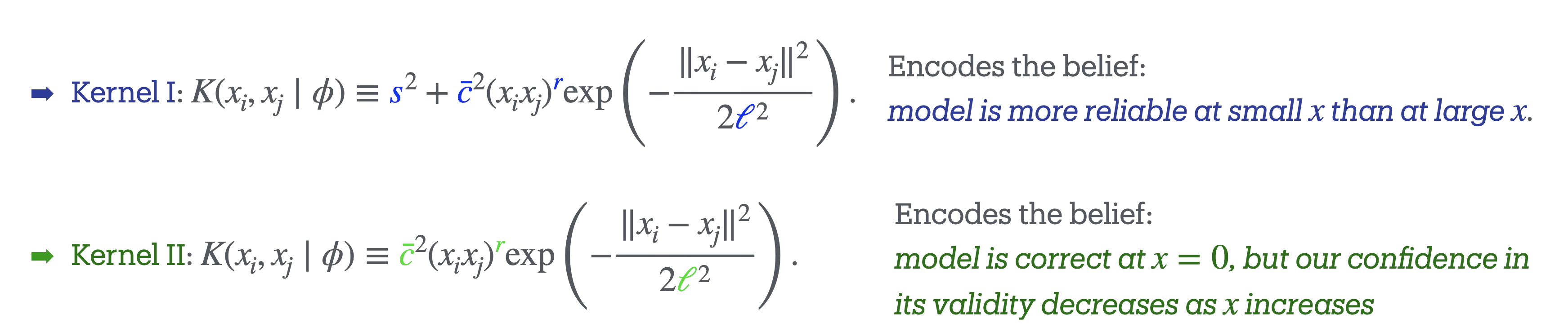
Fig. 11.5 GP kernels \(\texttt{I}\) and \(\texttt{II}\) for the balldrop analysis.

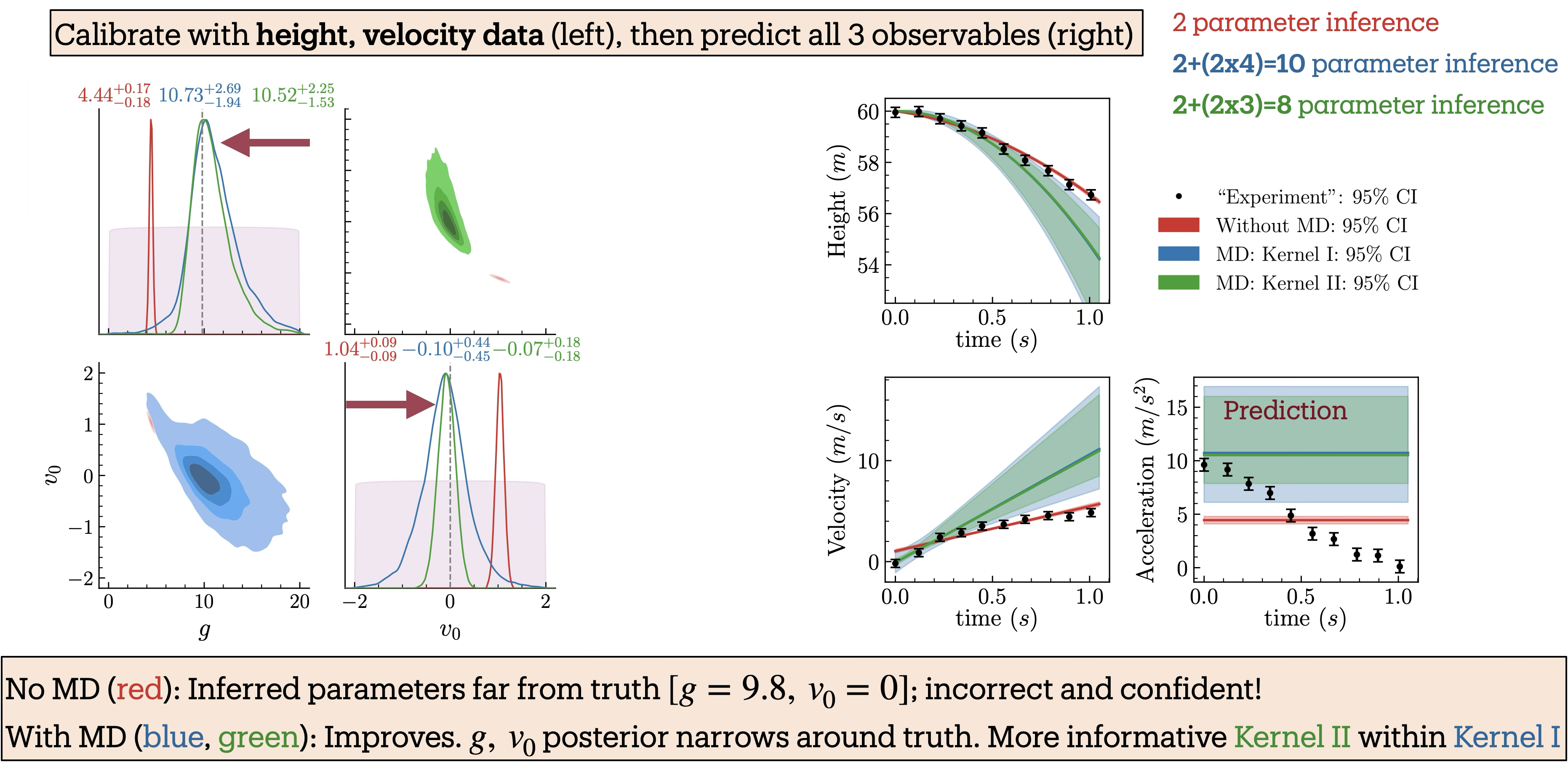
Fig. 11.6 Balldrop analysis with both the height and velocity measurements.

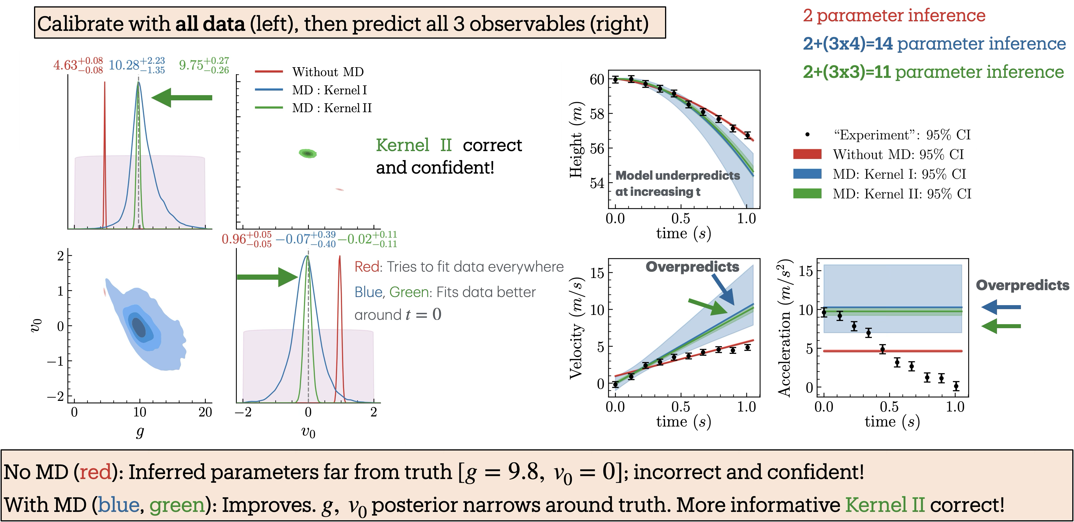
Fig. 11.7 Balldrop analysis with height, velocity, and acceleration measurements.

The posteriors incorporating MD (blue and green) consistently cover the true values and become narrower as more observables are included. In particular, the posteriors with MD using Kernel \(\texttt{II}\) (green), which encodes strong prior information about the theory’s domain of validity, are consistently tighter, reflecting greater constraining power, yet remain consistent with those obtained using the more conservative Kernel \(\texttt{I}\) (blue). Remarkably, when acceleration data are included (Fig. 11.7), the posterior with Kernel \(\texttt{II}\) nearly recovers the true parameter values, even though the model predicts a constant acceleration that does not capture the observed decreasing trend in the data. In contrast, the posteriors from the inference without the MD term (red) deviate significantly from the truth and become increasingly narrow as more observables are added, resulting in model parameter estimates that are both incorrect and overconfident.

In the right panels of the figures, the mock experimental data are compared with the model predictions generated using the inferred parameter posteriors from the left panels. Notably, predictions with MD (blue, green) match the data at early times and deviate at later times, a behavior that directly results from incorporating prior knowledge about the theory’s domain of applicability into the covariance kernel. In contrast, predictions without MD (red) prioritize achieving the best fit to the data, leading to inaccurate and overconfident parameter estimates.