📥 Visualizing correlated Gaussian distributions

A multivariate Gaussian distribution for \(N\) dimensional \(\boldsymbol{x} = \{x_1, \ldots, x_N\}\) with \(\boldsymbol{\mu} = \{\mu_1, \ldots, \mu_N\}\), with positive-definite covariance matrix \(\Sigma\) is

\[ p(\boldsymbol{x}|\boldsymbol{\mu},\Sigma) = \frac{1}{\sqrt{\det(2\pi\Sigma)}} e^{-\frac{1}{2}(\boldsymbol{x}-\boldsymbol{\mu})^\intercal\Sigma^{-1}(\boldsymbol{x}-\boldsymbol{\mu})} \]

For the one dimensional case, it reduces to the familiar

\[ p(x_1|\mu_1,\sigma_1) = \frac{1}{\sqrt{2\pi\sigma_1^2}} e^{-\frac{(x_1-\mu_1)^2}{2\sigma_1^2}} \]

with \(\Sigma = \sigma_1^2\).

For the bivariate case (two dimensional),

\[\begin{split} \boldsymbol{x} = \pmatrix{x_1\\ x_2} \quad\mbox{and}\quad \boldsymbol{\mu} = \pmatrix{\mu_1\\ \mu_2} \quad\mbox{and}\quad \Sigma = \pmatrix{\sigma_1^2 & \rho_{12} \sigma_1\sigma_2 \\ \rho_{12}\sigma_1\sigma_2 & \sigma_2^2} \quad\mbox{with}\ 0 < \rho_{12}^2 < 1 \end{split}\]

and \(\Sigma\) is positive definite.

Questions to consider:

1. What does “positive definite” mean and why is this a requirement for the covariance matrix \(\Sigma\)?

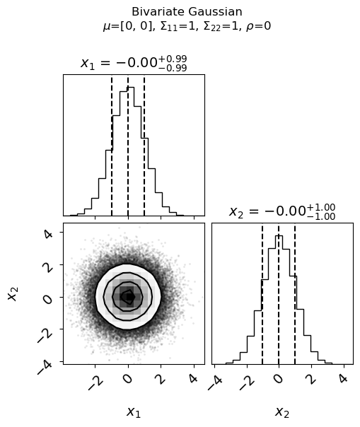
2. What is plotted in each part of the graph (called a “corner plot”)?

3. What effect does changing \(\mu_1\) (mu1) or \(\mu_2\) (mu2) have?

4. What effect does changing \(\sigma_1\) (var1) or \(\sigma_2\) (var2) have? What if the scales for \(x_1\) and \(x_2\) were the same?

5. What happens if \(\rho_{12}\) (rho) is equal to \(0\) then \(+0.5\) then \(-0.5\).

6. What happens if \(\rho_{12}\) (rho) is \(>1\) or \(< -1\)? Explain what goes wrong.

7. So what characterizes independent (uncorrelated) variables versus positively correlated versus negatively correlated?

import numpy as np
import matplotlib.pyplot as plt
import corner

def plot_bivariate_gaussians(mu1, mu2, var1, var2, rho, samples=100000):
    """
    Generates and plots samples from a 2D correlated Gaussian distribution 
    (also known as a bivariate normal distribution).
    
    Args:
        mu1 (float): Mean of the first dimension.
        mu2 (float): Mean of the second dimension.
        var1 (float): Variance of the first dimension.
        var2 (float): Variance of the second dimension.
        rho (float): Correlation coefficient between the dimensions.
    """
    # Create the mean vector and covariance matrix
    mean = np.array([mu1, mu2])
    cov = np.array([
        [var1, rho * np.sqrt(var1 * var2)],
        [rho * np.sqrt(var1 * var2), var2]
    ])

    # Generate samples from the multivariate normal distribution
    try:
        samples = np.random.multivariate_normal(mean, cov, size=samples)
    except np.linalg.LinAlgError:
        print("Invalid covariance matrix. Ensure `var1` and `var2` are positive.")
        return

    # Create the corner plot
    fig = corner.corner(samples, labels=[r'$x_1$', r'$x_2$'], 
                        quantiles=[0.16, 0.5, 0.84], 
                        show_titles=True, 
                        label_kwargs={"fontsize": 14},
                        title_kwargs={"fontsize": 14})
    # Adjust the fonts for the tick labels
    for ax in fig.get_axes():
      ax.tick_params(axis='both', labelsize=14)
    
    # Update the title with the current parameters
    fig.suptitle(
        f"Bivariate Gaussian\n$\mu$=[{mu1}, {mu2}], $\Sigma_{{11}}$={var1}, $\Sigma_{{22}}$={var2}, $\\rho$={rho}", 
        y=1.1)
    plt.show()

mu1 = 0
mu2 = 0
var1 = 1
var2 = 1
rho = 0

plot_bivariate_gaussians(mu1, mu2, var1, var2, rho)