35. Statistics concepts and notation#
“If your result needs a statistician then you should design a better experiment.”
—Ernest Rutherford
35.1. Notation#
Quantity |
General notation |
|---|---|
Conditional probability |
\(\cprob{A}{B}\) |
Covariance |
\(\cov{X}{Y}\) |
Distribution function |
\(P(x)\) |
Empty set |
\(\emptyset\) |
Event |
\(A\) |
Expectation value |
\(\expect{X}\) |
Likelihood function |
\(\mathcal{L}(\para)\) |
Model parameters |
\(\para\) |
Probability density function |
\(\p{x}\) |
Probability mass function |
\(\p{x}\) |
Probability measure |
\(\prob\) |
Random variable |
\(X\) |
Sample space |
\(S\) |
Standard deviation |
\(\std{X}\) |
Variance |
\(\var{X}\) |
35.2. Important definitions#
The set of all possible outcomes of an experiment is known as the sample space and is here denoted by \(S\). We can think of events \(A\) as subsets of the sample space.
Whenever \(A\) and \(B\) are events that we are interested in, then we can also reasonably concern ourselves with the events (\(A \cap B\)), (\(A \cup B\)), and (\(\bar{A}\)) which correspond to (\(A\) and \(B\)), (\(A\) or \(B\)), and (not \(A\)), respectively.
The probability measure#
Definition 35.1 (Probability measure)
A probability measure is a function \(\prob : A \to [0,1]\) satisfying
\(\prob (S)=1\)
\(\prob (\emptyset)=0\)
If \(A_1, A_2, \ldots A_n\) is a collection of disjoint events, such that \(A_i \cap A_j = \emptyset\) for all \(i \neq j\), then \(\prob \left( \cup_{i=1}^n A_i \right) = \sum_{i=1}^n \prob (A_i)\).
In particular, we will often consider the probability for two events to be true \(\prob (A \cap B)\). For brevity, we will often use the simpler notation \(\prob (A, B)\).
Definition 35.2 (Independent events)
Two events \(A\) and \(B\) are independent if
Definition 35.3 (Conditional probability)
Given \(\prob (A) > 0\) we define the conditional probability of \(B\) given \(A\) as
Alternatively this can be expressed via the product rule of probability theory
Given \(\prob (A) > 0\) we have that \(A\) and \(B\) are independent if and only if \(\cprob{B}{A} = \prob (B)\).
The total law of probability can be obtained from the disjoint-union property of Definition 35.1 and the product rule (35.3). Consider a partition \(B_1, B_2, \ldots, B_n\) of the complete state space (meaning that \(B_i \cap B_j = \emptyset\) for all \(i \neq j\) and \(\sum_{i=1}^n \prob (B_i) = 1\)) such that \(\prob (B_i) > 0\) for all \(i\). Then
This process of summing over all possible states of an event in a joint probability to obtain the marginal probability of the other event is known as marginalization.
A simple example of this law would be the statement
The total probability that it rains tomorrow is the sum of the probability that it rains tomorrow and that it rains today plus the probability that it rains tomorrow and not today.
Each of those joint probabilities can be factorized according to the product rule. For example, the probability that it rains tomorrow and that it rains today is the conditional probability of raining tomorrow given that it rains today times the probability that it rains today.
The point here is that the total probability of rain tomorrow is the sum of those two terms since the two events “it rains today” and “it does not rain today” form a complete and exhaustive partition of outcomes of the experiment “will it rain today?”.
Random variables: probability distribution and density#
Let us introduce the concept of random variables and use those to introduce probability distribution and density functions.
Definition 35.4 (Random variable and distribution function)
A random (or stochastic) variable is a function \(X: S \to \mathbb{R}\).
The distribution function \(P\) for a random variable \(X\) is the function \(P : \mathbb{R} \to [0,1]\), given by
We can write \(P_X(x)\) where it is necessary to emphasize the role of \(X\).
Definition 35.5 (Joint probability distribution)
The joint distribution function of a vector \(\boldsymbol{X}\) of random variables \(\boldsymbol{X} = (X_1, X_2, \ldots, X_n)\) is the function \(P : \mathbb{R}^n \to [0,1]\) given by
We can write \(P_{\boldsymbol{X}}\) where it is necessary to emphasize the role of \(\boldsymbol{X}\).
For random variables that are continuous it will be very useful to work with probability densities. Let us define those, starting however with the corresponding quantity (probability mass) for discrete random variables.
Definition 35.6 (Probability mass function)
The random variable \(X\) is called discrete if it takes values only in some countable subset \(\{ x_1, x_2, \ldots\}\) of \(\mathbb{R}\). The function \(p : \mathbb{R} \to [0,1]\), given by
is known as its probability mass function. Again, we can write \(p_X(x)\) where it is necessary to emphasize the role of \(X\).
The joint probability mass function of a random vector \(\boldsymbol{X} = (X_1, X_2, \ldots, X_n)\) is the function \(p : \mathbb{R}^n \to [0,1]\) given by
Definition 35.7 (Probability density function)
The random variable \(X\) is called continuous if its distribution function can be expressed as
for some integrable function \(p : \mathbb{R} \to [0,\infty)\) called the probability density function (PDF). Again, we can write \(p_X(x)\) where it is necessary to emphasize the role of \(X\).
The joint probability density function of a random vector \(\boldsymbol{X} = (X_1, \ldots, X_n)\) of continuous variables is the function \(p : \mathbb{R}^n \to [0,\infty)\) given by
Note that we will not differentiate in notation between probability mass and density functions as the context should make it clear whether it describes the probability density of a discrete or continuous variable. We will also refer to both as a PDF.
While discrete examples tend to be simpler, situations with continuous variables are more common in physics.
Following the above definition, there are some properties that all PDFs must have. Here we list some important ones using the simplest example of a single (continuous) random variable \(X\)
The first one is positivity
(35.11)#\[\begin{equation} 0 \leq p(x). \end{equation}\]Naturally, it would be nonsensical for any of the values of the domain to occur with a probability density less than \(0\).
Also, the PDF must be normalized. That is, all the probabilities must add up to one. The probability of anything to happen is always unity. For a continuous PDF this condition is
(35.12)#\[\begin{equation} \int_{-\infty}^\infty p(x)\,dx = 1. \end{equation}\]The corresponding condition for a discrete PDF is \(\sum_{i} p(x_i) = 1\).
The probability for any specific outcome \(x\) of a continuous variable \(X\) is zero
(35.13)#\[\begin{equation} \prob (X=x) = 0, \qquad \text{for all } x \in \mathbb{R}, \end{equation}\]since probabilities will be computable from the integral measure \(p(x) dx\) and \(\prob (X=x)\) would correspond to \(dx \to 0\).
Instead it makes more sense to discuss the probability for the outcome being within a domain. E.g., for the univariate case we can quantify
(35.14)#\[\begin{equation} \prob (a \leq X \leq b) = \int_a^b p(x) dx. \end{equation}\]From which we can also note that PDFs are not dimensionless objects. We must have \([p(x)] = [x]^{-1}\) for the integral to produce a dimensionless probability.
These properties can be generalized to the multivariate case \(p(x_1, x_2, \ldots)\).
For the multivariate case we also introduce the important concepts of marginalization and independence .
Property 35.1 (Marginal density functions)
Given a joint density function \(p(x,y)\) of two random variables \(X\) and \(Y\), the (marginal) probability density function of \(X\) is obtained via marginalization
and vice versa for \(p(y)\).
Marginalization is a very powerful technique as it allows to extract probabilites for a variable of interest when dealing with multivariate problems.
Property 35.2 (Independence)
Two random variables \(X\) and \(Y\) are independent if (and only if) the joint density function factorizes
Suppose that \(X\) and \(Y\) have the joint distribution function \(p(x,y)\). We wish to discuss the conditional probability distribution of \(Y\) given that \(X\) takes the value \(x\). However, we need to be careful since the event \(X=x\) has zero probability. Instead, we can consider the event \(x \leq X \leq x+dx\) which leads to the following definition
Definition 35.8 (Conditional probability-distribution)
The conditional distribution function of \(Y\) given \(X=x\) is
for any \(x\) such that \(p_X(x) > 0\).
The integrand is then defined as the conditional PDF
for any \(x\) such that \(p_X(x)>0\).
Note
Probability densities are usually introduced in the context of random variables (as we did here). However, from the Bayesian viewpoint, probabilities are used more generally to describe our state of knowledge. This means, for example, that we will use probability densities to quantify our knowledge of physics model parameters. Such a PDF would not make sense in an approach that requires randomness in considered variables.
Expectation values and moments#
Definition 35.9 (Expectation value)
Let \(h(x)\) be an arbitrary continuous function on the domain \(\mathbb{R}\) of the continuous, random variable \(X\) whose PDF is \(p(x)\). We define the expectation value of \(h\) with respect to \(p\) as follows
The corresponding definition for a discrete variable \(X\) is
Note that we usually drop the index \(p\) and just write \(\mathbb{E}[h]\).
A particularly useful class of expectation values are the moments. The \(n\)-th moment of the PDF \(p(x)\) is defined as follows
The zero-th moment \(\mathbb{E}[1]\) is just the normalization condition of \(p\). The first moment, \(\mathbb{E}[X]\), is called the mean of \(p\) and is often denoted by the greek letter \(\mu\)
for a continuous distribution and
for a discrete distribution.
Qualitatively it represents the average value of the PDF and is therefore sometimes called the expectation value of \(p(x)\).
Central moments: Variance and Covariance#
Another special case of expectation values is the set of central moments, with the \(n\)-th central moment defined as
The zero-th and first central moments are both trivial; equal to \(1\) and \(0\), respectively. Instead, the second central moment is of particular interest.
Definition 35.10 (Variance)
The variance of a random variable \(X\) is usually denoted \(\sigma^2\) or Var\((X)\) and is defined as
We note that
The positive square root of the variance, \(\sigma = +\sqrt{\sigma^2}\) is called the standard deviation of \(p\). It is the root-mean-square (RMS) value of the deviation of the PDF from its mean value, interpreted qualitatively as the “spread” of \(X\) around its mean.
When dealing with two random variables it is useful to introduce the covariance
Definition 35.11 (Covariance and correlation)
The covariance of two random variables \(X\) and \(Y\) is usually denoted \(\sigma_{XY}^2\) or \(\text{Cov}(X,Y)\) and is defined as
The correlation coefficient of \(X\) and \(Y\) is defined as
as long as the variances are non-zero.
You can show that the correlation coefficient is \(-1 \leq \rho \leq 1\). In particular, the diagonal covariance is the variance and therefore \(\rho_{XX} = 1\).
Two variables \(X\) and \(Y\) are called uncorrelated if Cov\((X,Y)=0\). Note that the independence property of Eq. (35.16) implies that two independent variables are always uncorrelated. However, the converse is not necessarily true.
35.3. Important distributions#
Let us consider some important, univariate distributions.
The uniform distribution#
The first one is the most basic PDF; namely the uniform distribution. This distribution is constant in a range \([a,b]\) and zero elsewhere. Thus, when a random variable \(X\) is uniformly distributed on \([a,b]\) we can write \(X \sim \mathcal{U}([a,b])\) with
For \(a=0\) and \(b=1\) we have the standard uniform distribution
Note that these functions correspond to properly normalized PDFs such that they give a total probability of one when integrated over \(x \in (-\infty,\infty)\).
Gaussian distribution#
The second one is the univariate Gaussian distribution (or normal distribution). A random variable \(X \sim \mathcal{N}(\mu,\sigma^2)\) is normally distributed with mean value \(\mu\) and standard deviation \(\sigma\) with
the corresponding PDF. If \(\mu=0\) and \(\sigma=1\), it is called the standard normal distribution
We sometimes denote distributions using a notation like \(\mathcal{N}(x|\mu,\sigma^2)\). This should be understood as a variable \(x\) being normally distributed with mean \(\mu\) and variance \(\sigma^2\).
Multivariate Gaussian distribution#
The univariate Gaussian distribution can be generalized to a multivariate distribution. A multivariate random variable \(\boldsymbol{X} \sim \mathcal{N}(\boldsymbol{\mu},\boldsymbol{\Sigma})\) is normally distributed with mean vector \(\boldsymbol{\mu} \in \mathbb{R}^k\) and covariance matrix \(\boldsymbol{\Sigma} \in \mathbb{R}^{k \times k}\) with
This distribution only exists for a positive definite covariance matrix \(\boldsymbol{\Sigma}\).
35.4. Quick introduction to scipy.stats#
The scipy.stats module contains a large number of probability distributions, summary and frequency statistics, correlation functions statistical tests, and more. If you google scipy.stats, you’ll likely get the manual page as the first hit: https://docs.scipy.org/doc/scipy/reference/stats.html. Here you’ll find a long list of the continuous and discrete distributions that are available for creating random variables, followed (scroll way down) by different methods (functions) to extract properties of a distribution (called Summary statistics) and to perform many other statistical tasks.
Follow the link for any of the distributions (your choice!) to find its mathematical definition, some examples of how to use it, and a list of methods. Some methods of particular interest are:
mean()- Mean of the distribution.median()- Median of the distribution.pdf(x)- Value of the probability density function at x.rvs(size=numpts)- generate numpts random values of the pdf.interval(alpha)- Endpoints of the range that contains alpha percent of the distribution.
Code example#
import scipy.stats as stats

# Define a normally distributed random variable with mean=1.0 and standard deviation = 2.0
my_norm_rv = stats.norm(loc=1.0, scale=2.0)

# Extract and print the mean and variance
print(f'The mean is {my_norm_rv.mean():3.1f}')
print(f'The variance is {my_norm_rv.var():3.1f}')

# The 68% credible interval (approximately one sigma)
(min68,max68) = my_norm_rv.interval(0.68)
print(f'The 68% credible interval is [{min68:4.2f},{max68:4.2f}]')

# Draw five random samples. Note that the last output will be printed.
my_norm_rv.rvs(size=5)
The mean is 1.0
The variance is 4.0
The 68% credible interval is [-0.99,2.99]
array([ 1.48831029, -0.0109919 , 0.2036921 , -0.51890728, -3.04380656])
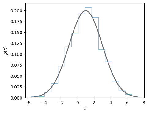
Create a plot to compare the line shape of the PDF with a histogram of a large number of samples from the PDF.
import matplotlib.pyplot as plt
import numpy as np
fig, ax = plt.subplots(nrows=1, ncols=1, **{"figsize":(5,4)})
x = np.linspace(my_norm_rv.ppf(0.001),
                my_norm_rv.ppf(0.999), 1000)
ax.plot(x, my_norm_rv.pdf(x),
       'k-', lw=2, alpha=0.6, label='pdf')
r = my_norm_rv.rvs(size=1000)
ax.hist(r, density=True, histtype='step', bins=16, alpha=0.5)
ax.set_xlabel(r'$x$')
ax.set_ylabel(r'$p(x)$');
(Pseudo) random number generator#
Random numbers generated by a computer are, in fact, not random at all. They are deterministically determined from a sequence of numbers that look random. The method to generate this sequence is known as a pseudo random number generator (PRNG), but will not be described here.
The scipy.stats module uses numpy functionality to generate random numbers and sample the distribution for a random variable. In fact, many of the standard distributions are built into numpy and if all you need is fast sampling of random numbers then you can often use numpy directly without the need for scipy.stats.
The lack of true randomness can be turned into a feature since it allows for experimentation, reproducibility and unit testing of code that uses stochastic modelling. The sequence of random numbers is determined by: (i) the choice of PRNG algorithm, and (ii) a seed to start the generation. Therefore, we can generate the same random numbers in two different runs by specifying the same PRNG and seed. In numpy the recommended procedure for random number sampling is to create a Generator instance with default_rng and call the relevant methods as attributes to this instance. In the code below, we illustrate this procedure to collect five samples from a standard normal distribution using both numpy and scipy.stats. You should get the same output if you run this code locally.
import numpy as np
import scipy.stats as stats
# seed number
seed=42
# Generator instance initialized with the seed
rng = np.random.default_rng(seed)
print(f'numpy samples from N(0,1) with {rng} and seed={seed}: ')
# Use numpy to collect samples from a standard normal
np_random_numbers = rng.normal(loc=0, scale=1, size=5)
print(np_random_numbers)

# The same with scipy.stats
# Create the random variable
my_norm_rv = stats.norm(loc=0.0, scale=1.0)
# sample, using the same PRNG and seed as before
rng = np.random.default_rng(seed)
print(f'scipy.stats samples from N(0,1) with {rng} and seed={seed}: ')
stats_random_numbers = my_norm_rv.rvs(size=5,random_state=rng)
print(stats_random_numbers)
numpy samples from N(0,1) with Generator(PCG64) and seed=42:
[ 0.30471708 -1.03998411  0.7504512   0.94056472 -1.95103519]
scipy.stats samples from N(0,1) with Generator(PCG64) and seed=42:
[ 0.30471708 -1.03998411  0.7504512   0.94056472 -1.95103519]
35.5. Point estimates and credible regions#
We will use PDFs to quantify the strength of our inference processes. However, one might be in a situation where it is desirable to summarize the information contained in a PDF in a single (or a few) numbers. This is not always easy, but some common choices are listed here.
Mean, median, mode#
The values of the mode, mean, and median can all be used as point estimates for the “most probable” value of \(X\). The mode is the position of the peak of the PDF, the mean was defined in Eq. (35.22), while the median is the value \(\mu_{1/2}\) for which \(P(\mu_{1/2}) = 0.5\). For some PDFs, these metrics will all be the same as exemplified in the first and last panel of Fig. 35.1. For others, such as exemplified in the middle panel, they will not.
Let us consider three example PDFs that illustrate some of the features of the different point estimates and the problems that might occur.
fig_point, axs = plt.subplots(nrows=1, ncols=3, sharey=True, **{"figsize":(10,4)})
my_rvs = [stats.norm(loc=5,scale=4),stats.invgamma(1.5, loc=0.0, scale=5.0),stats.beta(0.95, 0.95, scale=10)]
x = np.linspace(-5,30,10000)
for ax, my_rv in zip(axs,my_rvs):
    ax.plot(x, my_rv.pdf(x),
           'k-', lw=2, alpha=0.6)
    # Find and plot the mean
    ax.axvline(x=my_rv.mean(),ls='--',c='b',label='mean')
    # Find and plot the median
    ax.axvline(x=my_rv.median(),ls='-.',c='r',label='median')
    # Find and plot the mode(s)
    modes = np.logical_and(my_rv.pdf(x[1:-1])>my_rv.pdf(x[:-2]),
                           my_rv.pdf(x[1:-1])>my_rv.pdf(x[2:]))
    for xmode in x[1:-1][modes]:
        ax.axvline(x=xmode,ls=':',c='k',label='mode')
    ax.set_xlabel(r'$x$')
    if ax==axs[0]:
        ax.set_ylabel(r'$p(x)$')
        ax.legend(loc='best');
    if not ax==axs[1]:
        ax.set_xlim(-5,15)

from myst_nb import glue
glue("pointestimates_fig", fig_point, display=False)
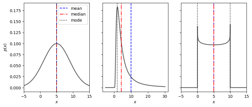
Fig. 35.1 The mean, median and modes(s) for some exampls PDFs. For some PDFs, several or all of these metrics are the same. For others they are not. The position of the mean is largely affected by long tails as illustrated in the middle panel. The PDF in the right panel has two modes (it is bimodal). Although no shuch example is shown here, there are PDFs for which the mean is not defined.#
Discuss
Which point estimate do you consider most representative for the different PDFs?
Credible regions#
The integration of the PDF over some domain translates into a probability. It is therefore possible to identify regions \(\mathbb{D}_P\) for which the integrated probability equals some desired value \(P\), i.e.,
This allows to make statements such as: “There is a 50% probability that the parameters are found within the domain \(\mathbb{D}_{0.5}\)””. However, the identification of such a domain is not unique. Two popular choices are
Highest-density regions (HDR)
The HDR is the smallest possible domain that gives the desired probability mass. That is
(35.35)#\[\begin{equation} p(\boldsymbol{x}) \geq p(\boldsymbol{y}), \quad \text{when } \boldsymbol{x} \in \mathbb{D}_P \text{ and } \boldsymbol{y} \notin \mathbb{D}_P. \end{equation}\]Equal-tailed interval (ETI)
For a univariate PDF we can define an interval \([a,b]\) such that \(\int_a^b p(x) dx = P\) and the probability mass on either side (the tails) are equal. The end points of this ETI fulfil
(35.36)#\[\begin{equation} P(a) = 1-P(b) = \frac{1-P}{2}. \end{equation}\]
Discuss
How would you describe a multimodal PDF using these metrics?
Let us again consider the three example PDFs from above.
fig_CR, axs = plt.subplots(nrows=1, ncols=3, sharey=True, **{"figsize":(10,4)})
for ax, my_rv in zip(axs,my_rvs):
    ax.plot(x, my_rv.pdf(x),
           'k-', lw=2, alpha=0.6)
    # Find and plot the 68% credible interval
    (min68,max68) = my_rv.interval(0.68)
    ax.axvline(x=min68,ls='--',c='g')
    ax.axvline(x=max68,ls='--',c='g')
    ax.fill_between(x,my_rv.pdf(x),where=np.logical_and(x>min68,x<max68), color='g',alpha=0.2)
    # Find and plot the 90% credible interval
    (min90,max90) = my_rv.interval(0.90)
    ax.axvline(x=min90,ls=':',c='g')
    ax.axvline(x=max90,ls=':',c='g')
    ax.fill_between(x,my_rv.pdf(x),where=np.logical_and(x>min90,x<max90), color='g',alpha=0.1)
    ax.set_xlabel(r'$x$')
    if ax==axs[0]:
        ax.set_ylabel(r'$p(x)$');
    if not ax==axs[1]:
        ax.set_xlim(-5,15)
    glue("credibleregions_fig", fig_CR, display=False)
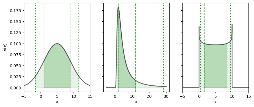
Fig. 35.2 The 68/90 percent credible regions of some example PDFs are shown in dark/light shading. These are all equal-tailed intervals.#
Let us also look at a multivariate PDF. The example below is a bivariate normal distribution with non-zero off-diagonal covariance. It is represented by a so called corner plot of a large number of samples. The bivariate distribution is shown in the lower left panel, while the two marginal ones are shown on the diagonal.
mean=[0.5,1]
cov = np.array([[1,-1],[-1,4]])
my_multinorm_rv=stats.multivariate_normal(mean=mean,cov=cov)
x1x2=my_multinorm_rv.rvs(size=100000)

# We use the prettyplease package from
# https://github.com/svisak/prettyplease
# which is in the ../Utils directory
import sys
import os
# Adding ../Utils/ to the python module search path
sys.path.insert(0, os.path.abspath('../Utils/'))

import prettyplease.prettyplease as pp

fig_x1x2 = pp.corner(x1x2, bins=50, labels=[r'$x_1$',r'$x_2$'],
                          quantiles=[0.16, 0.84], levels=(0.68,0.9),linewidth=1.0,
                          plot_estimates=True, colors='green', n_uncertainty_digits=2,
                          title_loc='center', figsize=(5,5))
glue("bivariate_fig", fig_x1x2, display=False)
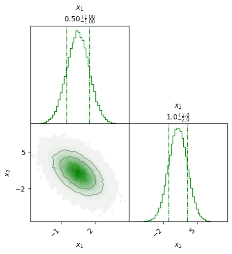
Fig. 35.3 A corner plot of a bivariate normal PDF. The 68% and 90% credible regions are indicated by level curves in the lower left panel. Note the anti-correlation between the two variables (the correlation coefficient is \(\rho_{12}=-0.5\)). The marginal distributions for \(x_1\) and \(x_2\) are shown in the diagonal panels with the dashed lines indicating the corresponding 68% credible intervals. Note that the marginal PDFs are univariate normal distributions.#
35.6. Types of probability#
As we have shown, we construct a probability space by assigning a numerical probability in the range [0,1] to events (sets of outcomes) in some space.
When outcomes are the result of an uncertain but repeatable process, probabilities can always be measured to arbitrary accuracy by simply observing many repetitions of the process and calculating the frequency at which each event occurs. These frequentist probabilities have an appealing objective reality to them.
Discuss
How might you assign a frequentist probability to statements like:
The electron spin is 1/2.
The Higgs boson mass is between 124 and 126 GeV.
The fraction of dark energy in the universe today is between 68% and 70%.
The superconductor Hg-1223 has a critical temperature above 130K.
The answer is that you cannot (if we assume that these are universal constants), since that would require a measurable process whose outcomes had different (random) values for the corresponding universal constant. Or maybe you could if you had access to a number of multiverses with different universal constants in each.
The inevitable conclusion is that the statements we scientists are most interested in cannot be assigned frequentist probabilities.
However, if we allow probabilities to also measure our subjective “degree of belief” in a statement, then we can use the full machinery of probability theory to discuss more interesting statements. These are called Bayesian probabilities. Note that such probabilities are always conditional in the sense that they are statements based on given information.
Roughly speaking, the choice is between:
- Frequentist statistics
objective probabilities of uninteresting statements.
- Bayesian statistics
subjective probabilities of interesting statements.
35.7. Exercises#
Exercise 35.1 (Random and colorblind)
The gene responsible for color blindness is located on the X chromosome. In other words, red-green color blindness is an X-linked recessive condition and is much more common in males (with only one X chromosome). According to the Howard Hughes medical institute about 7% of men and 0.4% of women are red-green colorblind. Furthermore, sccording to SCB, the Swedish population is 50,3% male and 49,7% female. What is the probability that a person selcted at random is colorblind?
Exercise 35.2 (Conditional discrete probability mass function)
The joint probability mass function of the discrete variables \(X,Y\) is
Find the conditional probability mass function \(\pdf{y}{x}\).
Verify that it is properly normalized.
Exercise 35.3 (Conditional probability for continuous variables)
The continuous random variables \(X,Y\) have the joint density
Find the probability \(\cprob{Y<2}{X=5}\).
Exercise 35.4 (Conditional expectation)
Assume that the continuous random variables \(X,Y\) have the joint density
Find the conditional expectation \(\expect{Y \vert X=x}\).
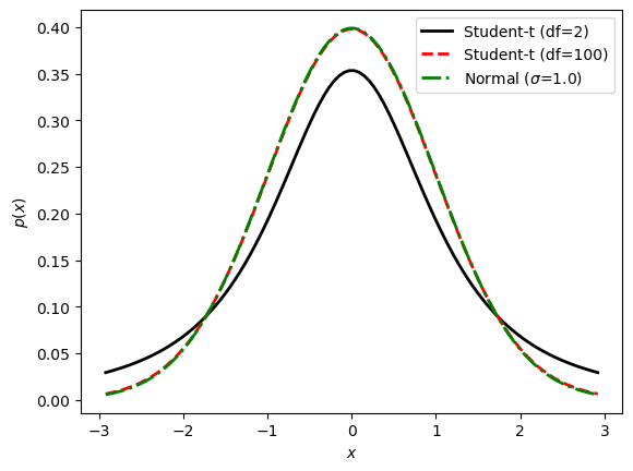
Exercise 35.5 (Scipy.stats)
Use scipy.stats to
Find and print the mean and the variance;
Find and print the 68% credible region (equal-tail interval);
Draw and print 5 random samples;
Plot the pdf (including at least 90% of the probability mass);
for
A student-t distribution with \(\nu=2\) degrees-of-freedom;
A student-t distribution with \(\nu=100\) degrees-of-freedom;
A standard normal distribution;
in all cases with the mode at 0.0.
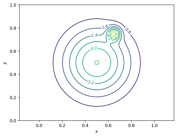
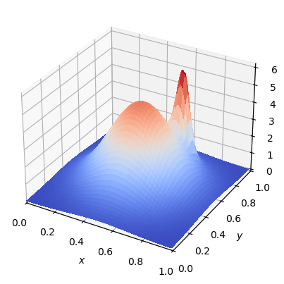
Exercise 35.6 (Bivariate pdf)
Consider the following (multimodal) bivariate pdf
with \(A_1=4.82033\), \(x_1=0.5\), \(y_1=0.5\), \(\sigma_1=0.2\), and \(A_2=4.43181\), \(x_2=0.65\), \(y_2=0.75\), \(\sigma_2=0.04\).
Consider the domain \(x,y \in [0,1]\) and use relevant python modules / methods to
Plot contour levels of this pdf (useful methods:
np.meshgridandplt.contour);Make a three-dimensional plot of the pdf (useful methods:
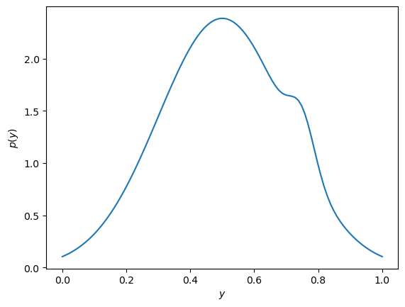
plt.subplots(subplot_kw={"projection": "3d"})andplt.plot_surface);Compute and plot the marginal pdf \(\p{y}\) (useful method:
scipy.integrate.quad)
35.8. Solutions#
Solution to Exercise 35.1 (Random and colorblind)
Let \(C\), \(M\), \(F\) denote the events that a random person is colorblind, male, and female, respectively. By the law of total probability
Solution to Exercise 35.2 (Conditional discrete probability mass function)
The conditional probability mass function can be obtained from the ratio
Let us therefore find the marginal probability mass function
Thus we get \(\pdf{y}{x} = \frac{(x+y)/18}{(x+1)/6} = \frac{x+y}{3(x+1)}\) for \(y \in \{0,1,2\}\).
We find that this pdf (over \(y\)) is properly normalized since
Solution to Exercise 35.3 (Conditional probability for continuous variables)
The desired probability is
To find the conditional density \(p_{Y|X}(y \vert x)\) we need the marginal one
for \(x > 0\). This gives
for \(0 < y < x\). Note that this is a uniform distribution for \(y\) given \(x\). Therefore
Solution to Exercise 35.4 (Conditional expectation)
We need the marginal density
to get the conditional one
The conditioned expectation is therefore
Solution to Exercise 35.5 (Scipy.stats)
See the code example in the hidden code block below.
Solution to Exercise 35.6 (Bivariate pdf)
See the code example in the hidden code block below.