28. *Convolutional Neural Networks#
Convolutional Neural Networks (CNNs) are very similar to ordinary Neural Networks, but are particularly adopted for image recognition.
They are made up of layers that have learnable weights and biases.
The inputs are operated on with dot products, typically followed by a non-linear activation function.
The whole network still expresses a single differentiable score function: from the raw image pixels on one end to class scores at the other.
And they still have a loss function (for example Softmax) on the last (fully-connected) layer.
Learning takes place via back propagation, gradient descent, etc.
What is the difference? CNN architectures make the explicit assumption that the inputs are images, which allows us to encode certain properties into the architecture. These then make the forward function more efficient to implement and vastly reduce the amount of parameters in the network.
Here we provide only a superficial overview.
28.1. Regular NNs don’t scale well to full images#
As an example, consider an image of size \(32\times 32\times 3\) (32 wide, 32 high, 3 color channels), so a single fully-connected neuron in a first hidden layer of a regular Neural Network would have \(32\times 32\times 3 = 3072\) weights. This amount still seems manageable, but clearly this fully-connected structure does not scale to larger images. For example, an image of more respectable size, say \(200\times 200\times 3\), would lead to neurons that have \(200\times 200\times 3 = 120,000\) weights.
We could have several such neurons, and the parameters would add up quickly! Clearly, this full connectivity is wasteful and the huge number of parameters would quickly lead to possible overfitting.
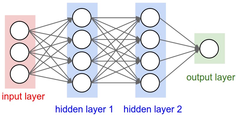
Fig. 28.1 A three-layer Neural Network.#
28.2. 3D volumes of neurons#
CNNs take advantage of the fact that the input consists of images and they constrain the architecture in a more sensible way.
In particular, unlike a regular Neural Network, the layers of a CNN have neurons arranged in 3 dimensions: width, height, depth. (Note that the word depth here refers to the third dimension of an activation volume, not to the depth of a full Neural Network, which can refer to the total number of layers in a network.)
To understand it better, the above example of an image with an input volume of activations has dimensions \(32\times 32\times 3\) (width, height, depth respectively).
The neurons in a layer will only be connected to a small region of the layer before it, instead of all of the neurons in a fully-connected manner. Moreover, the final output layer could for this specific image have dimensions \(1\times 1 \times 10\), because by the end of the CNN architecture we will reduce the full image into a single vector of class scores, arranged along the depth dimension.
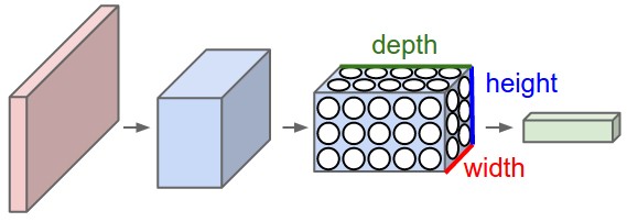
Fig. 28.2 A CNN arranges its neurons in three dimensions (width, height, depth), as visualized in one of the layers. Every layer of a CNN transforms the 3D input volume to a 3D output volume of neuron activations. In this example, the red input layer holds the image, so its width and height would be the dimensions of the image, and the depth would be 3 (Red, Green, Blue channels).#
28.3. Layers used to build CNNs#
A simple CNN is a sequence of layers, and every layer of a CNN transforms one volume of activations to another through a differentiable function. We use three main types of layers to build CNN architectures: Convolutional Layer, Pooling Layer, and Fully-Connected Layer (exactly as seen in regular Neural Networks). We will stack these layers to form a full CNN architecture.
The layers of a convolutional neural network arrange neurons in 3D: width, height and depth.
The input image is typically a square matrix of depth 3.
A convolution is performed on the image which outputs a 3D volume of neurons. The weights to the input are arranged in a number of 2D matrices, known as filters.
Each filter slides along the input image, taking the dot product between each small part of the image and the filter, in all depth dimensions. This is then passed through a non-linear function, typically the Rectified Linear (ReLu) function, which serves as the activation of the neurons in the first convolutional layer. This is further passed through a pooling layer, which reduces the size of the convolutional layer, e.g. by taking the maximum or average across some small regions, and this serves as input to the next convolutional layer.
Example: CNN architecture#
A simple CNN for image classification could have the architecture:
INPUT (\(32\times 32 \times 3\)) will hold the raw pixel values of the image, in this case an image of width 32, height 32, and with three color channels R,G,B.
CONV (convolutional )layer will compute the output of neurons that are connected to local regions in the input, each computing a dot product between their weights and a small region they are connected to in the input volume. This may result in volume such as \([32\times 32\times 12]\) if we decided to use 12 filters.
RELU layer will apply an elementwise activation function, such as the \(max(0,x)\) thresholding at zero. This leaves the size of the volume unchanged (\([32\times 32\times 12]\)).
POOL (pooling) layer will perform a downsampling operation along the spatial dimensions (width, height), resulting in volume such as \([16\times 16\times 12]\).
FC (i.e. fully-connected) layer will compute the class scores, resulting in volume of size \([1\times 1\times 10]\), where each of the 10 numbers correspond to a class score, such as among the 10 categories of the MNIST images we considered above . As with ordinary Neural Networks and as the name implies, each neuron in this layer will be connected to all the numbers in the previous volume.
Systematic reduction#
By systematically reducing the size of the input volume, through convolution and pooling, the network should create representations of small parts of the input, and then from them assemble representations of larger areas. The final pooling layer is flattened to serve as input to a hidden layer, such that each neuron in the final pooling layer is connected to every single neuron in the hidden layer. This then serves as input to the output layer, e.g. a softmax output for classification.
28.4. Transforming images#
CNNs transform the original image layer by layer from the original pixel values to the final class scores.
Observe that some layers contain parameters and other don’t. In particular, the CNN layers perform transformations that are a function of not only the activations in the input volume, but also of the parameters (the weights and biases of the neurons). On the other hand, the RELU/POOL layers will implement a fixed function. The parameters in the CONV/FC layers will be trained with gradient descent so that the class scores that the CNN computes are consistent with the labels in the training set for each image.
Example: The MNIST dataset#
The MNIST dataset consists of grayscale images with a pixel size of \(28\times 28\), meaning we require \(28 \times 28 = 724\) weights to each neuron in the first hidden layer.
If we were to analyze images of size \(128\times 128\) we would require \(128 \times 128 = 16384\) weights to each neuron. Even worse if we were dealing with color images, as most images are, we have an image matrix of size \(128\times 128\) for each color dimension (Red, Green, Blue), meaning 3 times the number of weights \(= 49152\) are required for every single neuron in the first hidden layer.
Setting it up#
It means that to represent the entire dataset of images, we require a 4D matrix or tensor. This tensor has the dimensions:
28.5. CNNs in brief#
In summary:
A CNN architecture is in the simplest case a list of layers that transform the image volume into an output volume (e.g. holding the class scores)
There are a few distinct types of layers (e.g. CONV/FC/RELU/POOL)
Each layer accepts an input 3D volume and transforms it to an output 3D volume through a differentiable function
Each layer may or may not have parameters (e.g. CONV/FC do, RELU/POOL don’t)
Each layer may or may not have additional hyperparameters (e.g. CONV/FC/POOL do, RELU doesn’t)
For more material on convolutional networks, we strongly recommend the slides of CS231 which is taught at Stanford University. Furthermore, Michael Nielsen’s book Neural Networks and Deep Learning is a very good read, in particular chapter 6 which deals with CNNs.