11.5. 📥 Model discrepancy example: The ball-drop experiment#
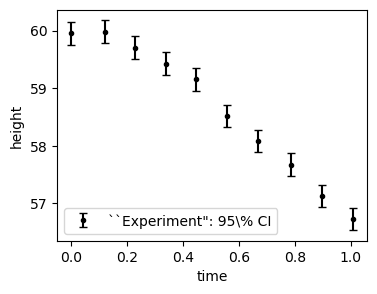
A ball is dropped from a tower of height \(h_0\) at initial time \(t_0=0\) with intial velocity \(v_0=0\). The height from the ground is recorded at discrete time points. Data is generated based on a model with drag, and includes uncorrelated Gaussian measurement errors. The aim is to extract the value of accelaration due to gravity, \(g\).
The problem is that the data is noisy and our theoretical model, which is simply free fall without drag, is incorrect. How can we best formulate our analysis such that the extraction of \(g\) is robust? I.e., that we get a distribution for \(g\) that covers the true answer with plausible uncertainty.
This notebook was created by Dr. Sunil Jaiswal in July, 2025.
Statistical formulation#
We will follow the article by Higdon et.al. The statistical equation accounting for model discrepancy is:
where \(x\) is the input vector (time in the case of the ball drop experiment) of length \(n\).
We shall denote the input domain as \(\{x_1,\cdots,x_n\}\in \chi_*\).
The above equation should be understood as an equation which holds on the range (set of all possible outcomes) of the probability distributions. It means that a sample drawn at a given \(x_i\) from the probability distributions \(\mathrm{pr}(y)\) should be equal to the sum of the sample drawn from each of the distributions \(\mathrm{pr}(\eta|{\boldsymbol \theta})\), \(\mathrm{pr}(\delta|{\boldsymbol \phi})\) and \(\mathrm{pr}(\epsilon|{\boldsymbol \sigma_{\boldsymbol \epsilon}})\).
Note that for given \(x_i\), \(\mathrm{pr}(\eta(x_i)|{\boldsymbol \theta}) = \delta(\eta(x_i)-\eta(x_i;{\boldsymbol \theta}))\) is deterministic since the model is deterministic given \({\boldsymbol \theta}\) (note: \(\delta\) is the Dirac delta function).
In Eq. (1), \(y(x_i)\) are vectors of the measured observables (velocity and height) at each input point \(x_i\).
The error in the measurement of \(y(x_i)\) is represented by \(\epsilon(x_i;{\boldsymbol \sigma_{\boldsymbol \epsilon}})\), which is assumed to be independently and identically distributed \(\sim N(0, {\boldsymbol \sigma_{\boldsymbol \epsilon}}^2)\) for each type of observable (velocity and height: \(\{\sigma_v, \sigma_h\} \in {\boldsymbol \sigma_{\boldsymbol \epsilon}}\)).
Note that \(\{\sigma_v, \sigma_h\}\) are fixed constants since we have assumed the distribution for each type of observable to be iid’s. We shall treat them as information `\(I\)’ whenever we write any probability distribution \(\mathrm{pr}(\bullet|\bullet,I)\), and will not state them explicitly.
\(\eta(x;{\boldsymbol \theta})\) denotes the observable predictions of the physics theory given the value of the parameters of the theory \(\{g, \sigma_{v_0}\}\in {\boldsymbol \theta}\).
The stochastic model \(\mathrm{pr}(\delta(x)|{\boldsymbol \phi}) = GP[0,\kappa(x, x';{\boldsymbol \phi})]\), accounts for model discrepancy (discrepancy between the physics model and reality) where \(\kappa\) is covariance kernel of the Gaussian Process (GP) with \(\{\bar{c}_v,\, l_v,\, \bar{c}_h,\, l_h\}\in {\boldsymbol \phi}\) representing the hyperparameters.
We define \(\{{\boldsymbol \theta}, {\boldsymbol \phi}\} \in {\boldsymbol \alpha}\) as a vector containing \({\boldsymbol \theta}\) and \({\boldsymbol \phi}\) for compact notation.
Theory#
Consider the drag force on the ball (sphere) for the true model to behave as
where \(v\) is magnitude of velocity \(\bf{v}\). The coefficients \(b\) and \(c\) are drag coefficients.
\(\bullet\) Equation of motion:
We have considerd the downward direction to be positive. Here \(\color{red}{m=1\, kg}\) is the mass of the sphere and \(\color{red}{g=9.8\, m/s^2}\) the acceleration due to gravity.
\(\bullet\) The equation for velocity can be written as \(m\frac{d v}{dt} = m g - b v- c v \sqrt{v^2}\). The last term is written such that it takes into account the direction of velocity in quadratic term. We need to solve the equations:
By default we consider the ball to have the initial height \(\color{red}{h_0=60\, m}\) at initial time \(\color{red}{t_0=0\,sec}\) with initial velocity \(\color{red}{v_0=0\, m/s^2}\).
Set plot style#
import matplotlib.pyplot as plt

# # Add the local CodeLocal directory to the path so Jupyter finds the module file.
# import sys
# sys.path.append('./CodeLocal')
# from setup_rc_params import setup_rc_params  # import from setup_rc_params.py in subdirectory CodeLocal

# setup_rc_params(presentation=True, constrained_layout=True, usetex=True, dpi=400)
Setup sampling with emcee and pocomc samplers#
import emcee
import pocomc   # uncomment here when using pocomc sampler
from multiprocess import Pool
from scipy.stats import uniform
import time
import os

# ================================ emcee sampler ==================================
def emcee_sampling(min_param, max_param, log_posterior,
                   nburn=2000, nsteps=2000, num_walker_per_dim=8, progress=False):
    """
    Function for sampling in parallel using emcee.

    Parameters:
      - min_param (list or array): minimum values parameters
      - max_param (list or array): maximum values parameters
      - log_posterior (callable): log posterior
      - nburn (int): "burn-in" period to let chains stabilize
      - nsteps (int): # number of MCMC steps to take after burn-in
      - num_walker_per_dim (int): number of walker per dimension
      - samples_save_dir (string): directory name in which the samples will be saved
      - progress (boolean): toggle the progress bar
    """
    if len(min_param) != len(max_param):
            raise ValueError(
                f"min_param and max_param must have the same length."
            )

    ndim = len(min_param)  # number of parameters in the model
    nwalkers = ndim * num_walker_per_dim  # number of MCMC walkers

    start_time = time.time()
    print(f"Starting MCMC sampling using emcee with {nwalkers} walkers in parallel...")

    # Generate starting guesses within the prior bounds
    starting_guesses =  min_param + (max_param - min_param) * np.random.rand(nwalkers,ndim)

    # Create a pool of workers using multiprocessing
    with Pool() as pool:
        # Pass the pool to the sampler
        sampler = emcee.EnsembleSampler(nwalkers,ndim,log_posterior,pool=pool)

        # "Burn-in" period
        pos, prob, state = sampler.run_mcmc(starting_guesses, nburn, progress=progress)
        sampler.reset()

        # Sampling period
        pos, prob, state = sampler.run_mcmc(pos, nsteps, progress=progress)

    # Collect samples
    samples = sampler.get_chain(flat=True)

    end_time = time.time()
    print(f"Sampling complete. Time taken: {(end_time - start_time)/60:.2f} minutes.")
    print(f"Mean acceptance fraction: {np.mean(sampler.acceptance_fraction):.3f} (in total {nwalkers*nsteps} steps)")
    print(f"Samples shape: {samples.shape}")

    return samples


# ================================ pocoMC sampler ==================================
def pocomc_sampling(min_param, max_param, log_posterior,
                    n_effective=2000, n_active=800, n_steps=None,
                    # n_prior=2048, n_max_steps=200,
                    n_total=5000, n_evidence=5000, ncores = -1
                   ):
    """
    This function is based on PocoMC package (version 1.2.1).
    pocoMC is a Preconditioned Monte Carlo (PMC) sampler that uses
    normalizing flows to precondition the target distribution.

    Parameters:
      - min_param (list or array): Minimum values parameters
      - max_param (list or array): Maximum values parameters
      - log_posterior (callable): Log posterior

      - n_effective (int): The effective sample size maintained during the run. Default: 2000.
      - n_active (int): Number of active particles. Default: 800. Must be < n_effective.
      - n_steps (int): Number of MCMC steps after logP plateau. Default: None -> n_steps=n_dim.
                       Higher values lead to better exploration but increases computational cost.
      - n_total (int): Total effectively independent samples to be collected. Default: 5000.
      - n_evidence (int): Number of importance samples used to estimate evidence. Default: 5000.
                          If 0, the evidence is not estimated using importance sampling.

      - ncores: Number of cores to use in sampling.
                  -1 (default): use all availaible cores
                   n (int): use n cores
    """

    # Generating prior range for pocomc
    priors = [uniform(lower, upper - lower) for lower, upper in zip(min_param, max_param)]
    prior = pocomc.Prior(priors)

    ndim = len(min_param)  # number of parameters in the model

    # --------------------------------------------------------------------------------------------
    # Try to get the allowed CPU count via affinity (works on Linux/Windows)
    try:
        available_cores = len(os.sched_getaffinity(0))# len(psutil.Process().cpu_affinity())
    except Exception:
        # On systems where affinity is not available (e.g., macOS), use total CPU count
        available_cores = os.cpu_count()

    # Validate that ncores is an integer and at least -1
    if not isinstance(ncores, int) or ncores < -1:
        raise ValueError("ncores must be an integer greater than or equal to -1. Specify '-1' to use all available cores.")

    if ncores == -1:
        # Use all available cores
        num_cores = available_cores
    elif ncores > available_cores:
        # Warn if more cores are requested than available and then use available cores
        warnings.warn(
            f"ncores ({ncores}) exceeds available cores ({available_cores}). Using available cores.",
            UserWarning
        )
        num_cores = available_cores
    else:
        num_cores = ncores
    # --------------------------------------------------------------------------------------------

    start_time = time.time()

    sampler = pocomc.Sampler(prior=prior, likelihood=log_posterior,
                                 n_effective=n_effective, n_active=n_active, n_steps=n_steps,
                                 # dynamic=True, n_prior=n_prior, n_max_steps=n_max_steps,
                                 pytorch_threads=None,  # use all availaible threads for training
                                 pool=num_cores
                                 )

    print(f"Starting sampling using pocomc in {num_cores} cores...")

    sampler.run(n_total=n_total,
                n_evidence=n_evidence,
                progress=True)


    # Generating the posterior samples
    # samples, weights, logl, logp = sampler.posterior() # Weighted posterior samples
    samples, _, _ = sampler.posterior(resample=True)  # equal weights for samples

    # Generating the evidence
    # logz, logz_err = sampler.evidence() # Bayesian model evidence estimate and uncertainty
    # print("Log evidence: ", logz)
    # print("Log evidence error: ", logz_err)

    # logging.info('Writing pocoMC chains to file...')
    # chain_data = {'chain': samples, 'weights': weights, 'logl': logl,
    #                 'logp': logp, 'logz': logz, 'logz_err': logz_err}

    end_time = time.time()
    print(f"Sampling complete. Time taken: {(end_time - start_time)/60:.2f} minutes.")
    print(f"Samples shape: {samples.shape}")

    return samples
Generate “experimental” observations for height#
import numpy as np
from scipy.integrate import odeint

def True_height(t, h0=60.0, v0=0.0,
                g=9.8, m=1.0, b=0.0, c=0.4):    # initial conditions
    """
    Height of a falling ball with linear + quadratic air drag.

    Parameters
    ----------
    t : float or 1-D array_like
        Time(s) at which to evaluate the height.
    h0, v0 : float, optional
        Initial height and velocity at time t = 0.
    g : float, optional
        Acceleration due to gravity (m s⁻²) (taken positive downward).
    m : float, optional
        Mass of the ball (kg).
    b, c : float, optional
        Linear and quadratic drag coefficients.

    Returns
    -------
    h : 1darray
        Height(s) at the requested time points (same shape as `t`).
    """

    def derivatives(y, _t):
        h, v = y
        dhdt = -v
        dvdt = g - (b*v)/m - (c*abs(v)*v)/m
        return [dhdt, dvdt]

    # Ensure we integrate from t0 out to the requested time(s)
    t = np.atleast_1d(t)
    times = np.concatenate(([t[0]], t))  # add t[0] to get solution at t=0
    sol = odeint(derivatives, [h0, v0], times)

    return sol[1:, 0]
np.random.seed(42)  # Set a random seed for reproducibility. Change 42 -> 0 for different seeds every time.

# Generate an array of time where height are observed -->
t_obs = np.linspace(0.0, 1.0, 10)
t_noise = np.random.uniform(1e-3, 1e-2, size = t_obs.shape)  # random noise added to time. helps in inversion of covariance matrix.
t_noise[0] = 0.0  # No noise for initial time
t_obs = np.round(t_obs + t_noise, decimals=4)


# Compute height of ball at these time steps -->
hexp_std = 0.1 # standard deviation of assumed gaussian noise as error of measurment
hexp_err = np.array([hexp_std]*len(t_obs))  # adding gaussian noise to observation of height
hexp_mean = np.random.normal(True_height(t_obs), hexp_err)    # observed height at input times
plt.figure(figsize=(4, 3))
plt.errorbar(t_obs, hexp_mean, yerr=[1.96*hexp_err, 1.96*hexp_err],
             fmt='o', markersize=3, capsize=3, color='black',
             label=f'``Experiment": 95\% CI')
plt.ylabel('height')
plt.xlabel('time')
plt.legend()

plt.show()
Define physics model#
def model_height(t, g, v0=0.0, h0=60.0):
    return np.atleast_1d(h0  - v0 * t - g * t**2 / 2.0 )

# def model_height(t, g, v0, h0=60.0):
#     f = True_height(t, h0=60.0, v0=v0, g=g, m=1.0, b=0.0, c=0.0)
#     return np.atleast_1d(f)
# model_height(t=t_obs, g = 9.8)
Define model discrepancy class#
from sklearn.preprocessing import StandardScaler
from scipy.spatial.distance import mahalanobis

class ModelDiscrepancy():
    def __init__(self, t_obs, hexp_mean, hexp_err, model_height, num_model_param, log_priors, MD = False, kernel_func = None):

        self.t_obs = t_obs
        self.hexp_mean = hexp_mean
        self.hexp_err = hexp_err
        self.model_height = model_height
        self.num_model_param = num_model_param
        self.log_priors = log_priors
        self.MD = MD
        self.kernel_func = kernel_func

        if self.MD:
            self.log_priors_model = self.log_priors[:self.num_model_param]
            self.log_priors_MDGP = self.log_priors[self.num_model_param:]
        else:
            self.log_priors_model = self.log_priors

        # standardize experimental data  ----->
        self.scaler = StandardScaler()
        self.hexp_mean_scaled = self.scaler.fit_transform(self.hexp_mean.reshape(-1, 1)).ravel()

        self.offset = float(self.scaler.mean_[0])
        self.scale = float(self.scaler.scale_[0])

        self.hexp_err_scaled = self.hexp_err / self.scale
    #=======================================================================

    def log_likelihood(self, theta, phi=[]):
        """
        Calculate the log-likelihood of a dataset given the mean and covariance matrix.

        Parameters:
            theta: 1D NumPy array containing model parameters.
            phi: 1D NumPy array containing GP kernel hyperparameters.

        Returns:
            Log-likelihood of the dataset.
        """

        if self.num_model_param == 1:
            g = theta[0]
            h = model_height(t = self.t_obs, g = g)
        elif self.num_model_param == 2:
            g, v0 = theta[0], theta[1]
            h = self.model_height(t = self.t_obs, g = g, v0 = v0)

        hmodel_scaled = (h - self.offset) / self.scale

        cov_exp = np.diag(self.hexp_err_scaled**2)

        if self.MD == False:
            cov_total = cov_exp
        else:
            X = self.t_obs.reshape(-1, 1)
            cov_total = self.kernel_func(X, X, *phi) + cov_exp

        k = len(self.t_obs)  # number of observables

        md2 = mahalanobis(self.hexp_mean_scaled, hmodel_scaled, np.linalg.inv(cov_total))**2

        # calculate the log-likelihood
        log_likelihood_value = -0.5 * (md2 + np.log(np.linalg.det(cov_total)) + k * np.log(2.0 * np.pi) )

        return log_likelihood_value
    #=======================================================================

    def log_posterior(self, theta_and_phi):
        """
        Calculate the log posterior = sum of log priors + log likelihood.

        Parameters
        ----------
        theta_and_phi : np.ndarray (1D)
            Combined array of model params (theta) and discrepancy params (phi) if MD=True.

        Returns
        -------
        float
            The log posterior value.
        """
        theta_and_phi = np.atleast_1d(theta_and_phi)

        if self.MD:
            theta = theta_and_phi[:self.num_model_param]
            phi = theta_and_phi[self.num_model_param:]

        else:
            theta = theta_and_phi
            phi = []

        # ----------------------------------------
        # Calculate log-prior for model parameters
        # ----------------------------------------
        log_prior_val = 0.0
        for i, prior_func in enumerate(self.log_priors_model):
            lp = prior_func(theta[i])
            if lp <= -1e5:
                return -1e30
            log_prior_val += lp

        # ------------------------------------------------------
        # If MD ==True, accumulate log-prior for phi as well
        # ------------------------------------------------------
        if self.MD:
            for i, prior_func in enumerate(self.log_priors_MDGP):
                lp = prior_func(phi[i])
                if lp <= -1e5:
                    return -1e30
                log_prior_val += lp

        # ------------------------
        # Calculate log-likelihood
        # ------------------------
        log_likelihood_val = self.log_likelihood(theta, phi)

        return log_prior_val + log_likelihood_val
Define priors#
from scipy.stats import beta

# Define function for general beta priors
def log_prior_param(param, alpha_val, beta_val, param_min, param_max):
    """
    Log prior for parameter based on a Beta distribution.
    """
    scale = param_max - param_min  # Rescaling factor

    if param_min < param < param_max:
        # Rescale param to the range [param_min, param_max]
        param_rescaled = (param - param_min) / scale

        prior = beta.pdf(param_rescaled, alpha_val, beta_val) / scale
        return np.log(prior)
    else:
        return -np.inf
model_param_bounds = np.array([[ 0.0,  20.0 ],
                               [-2.0 ,  2.0 ]])

# model_param_bounds = np.array([[ 0.0,  20.0 ]])  # When only model parameter is g -- That's all the change required in code

num_model_param = len(model_param_bounds)

# Define a list of log_prior functions for model parameters
log_prior_theta = [
    lambda param, i=i: log_prior_param(
        param, alpha_val=1.01, beta_val=1.01,  # for flat priors
        param_min=model_param_bounds[i][0], param_max=model_param_bounds[i][1]
    )
    for i in range(num_model_param)
]
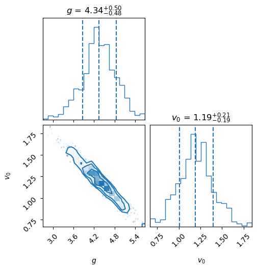
Without model discrepancy#
# Instantiate class  -->
MDC = ModelDiscrepancy(t_obs=t_obs, hexp_mean=hexp_mean, hexp_err=hexp_err,
                      model_height=model_height, num_model_param=num_model_param,
                      log_priors=log_prior_theta, MD = False, kernel_func = None)
from scipy import optimize

guess = model_param_bounds.mean(axis=1)

# Find Maximum likelihood value for parameters -->
nll = lambda *args: - MDC.log_likelihood(*args)
result = optimize.minimize(nll, guess,  method = 'Powell')
max_lik = result['x']
print(result)
print("\nMaximum likelihood value for parameters:", max_lik,"\n")


# Find MAP values for parameters -->
nlp = lambda *args: - MDC.log_posterior(*args)
result = optimize.minimize(nlp, guess,  method = 'Powell')
MAP = result['x']
print(result)
print("\nMAP values for parameters:", MAP)
 message: Maximum number of function evaluations has been exceeded.
 success: False
  status: 1
     fun: -8.556378888999681
       x: [ 3.977e+00  1.354e+00]
     nit: 83
   direc: [[ 7.342e-03  7.656e-05]
           [ 9.371e-03 -8.352e-04]]
    nfev: 2000

Maximum likelihood value for parameters: [3.97682437 1.35379069]
 message: Maximum number of function evaluations has been exceeded.
 success: False
  status: 1
     fun: -4.17801963736677
       x: [ 3.978e+00  1.353e+00]
     nit: 83
   direc: [[ 7.276e-03  1.052e-04]
           [ 9.307e-03 -8.065e-04]]
    nfev: 2000

MAP values for parameters: [3.97794526 1.35323281]
import corner

min_param = model_param_bounds[:,0]
max_param = model_param_bounds[:,1]
lab = [r'$g$', r'$v_0$']
Now do the sampling and plot the posteriors#
num_burn = 100  # 2000 is a minimum
num_steps = 100  # 2000 is a minimum

samples_WMD = emcee_sampling(min_param = min_param, max_param = max_param,
                         log_posterior = MDC.log_posterior,
                         nburn = num_burn, nsteps = num_steps, num_walker_per_dim = 8)

fig = corner.corner(samples_WMD, labels=lab, color='C0', quantiles=[0.16, 0.5, 0.84],
                   show_titles=True, title_kwargs={"fontsize": 12}, hist_kwargs={'density': True})
plt.show()
Starting MCMC sampling using emcee with 16 walkers in parallel...
Sampling complete. Time taken: 0.41 minutes.
Mean acceptance fraction: 0.714 (in total 1600 steps)
Samples shape: (1600, 2)
# # sampling with pocomc for consistency check --->

# n_effective_mltpl = 500
# n_active_mltpl = 150  # 0.3 x n_eff
# n_steps_mltpl = 2
# num_param = len(min_param)

# n_effective = n_effective_mltpl * num_param
# n_active = n_active_mltpl * num_param
# n_steps = n_steps_mltpl * num_param
# # print(n_effective, n_active, n_steps)

# n_total = 20000

# samples_WMD_poco = pocomc_sampling(min_param, max_param, MDC.log_posterior,
#                                   n_effective=n_effective, n_active=n_effective, n_steps=n_steps,
#                                   n_total=n_total, n_evidence=n_total)

# fig = corner.corner(samples_WMD_poco, labels=lab, color='C0', quantiles=[0.16, 0.5, 0.84],
#                    show_titles=True, title_kwargs={"fontsize": 12}, hist_kwargs={'density': True})
# plt.show()
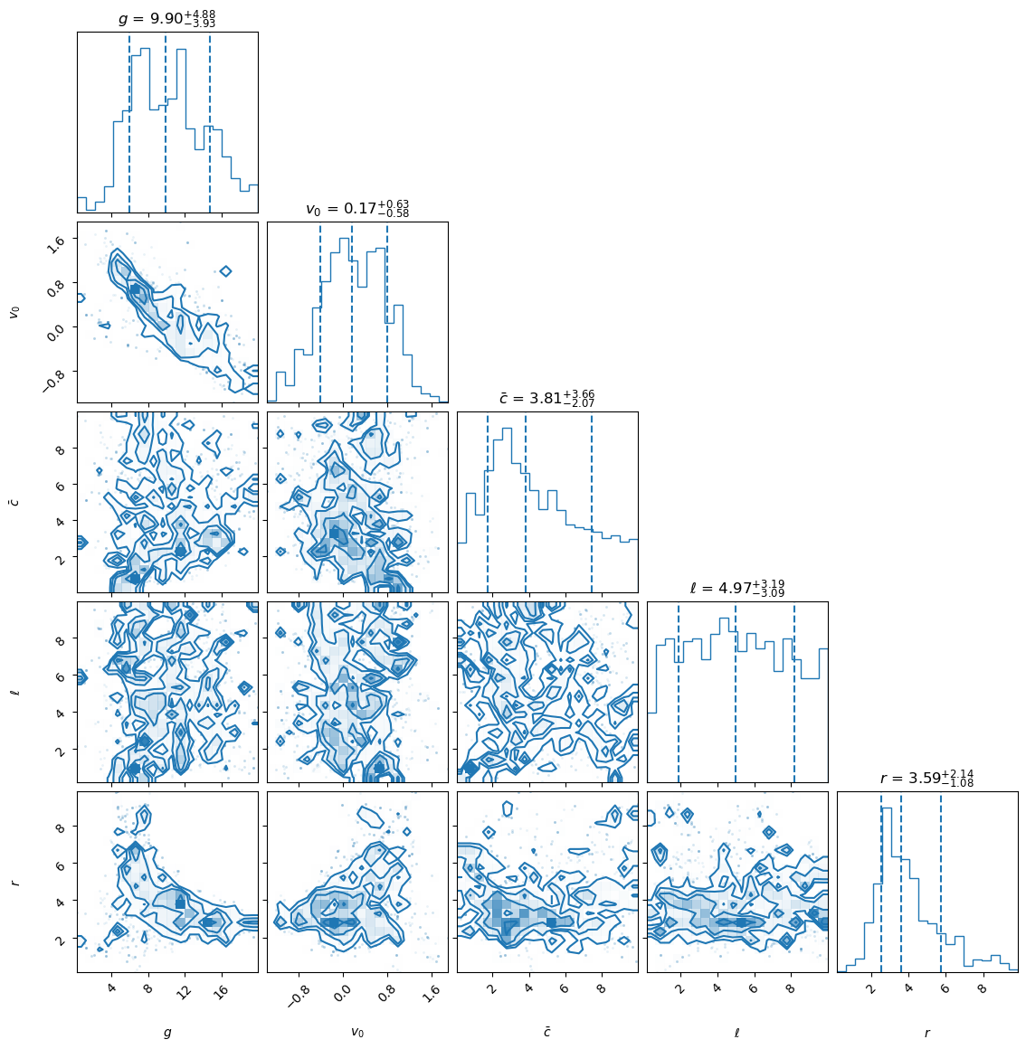
With model discrepancy#
from sklearn.gaussian_process.kernels import DotProduct, RBF

def MD_kernel(X1, X2, cbar, l, r, s):
    """
    Compute the covariance matrix using a custom kernel:
    K(X1, X2) = s^2 + cbar^2 * (X1 @ X2.T)^r * exp(-||X1 - X2||^2 / (2 * l^2)).

    This kernel serves as the core of the Model Discrepancy framework and should be modified
    to suit specific problems.

    Parameters:
        - X1 (numpy.ndarray): A matrix where each row represents an input vector.
        - X2 (numpy.ndarray): A matrix where each row represents an input vector.
        - cbar (float): The marginal variance parameter.
        - l (float): The length scale parameter for the RBF term.
        - r (float): The power applied to the dot product term.
        - s (float): A constant shift.

    Returns:
        - numpy.ndarray: A covariance matrix computed using the defined kernel.
    """
    # Compute the dot product term
    dot_product_term = np.dot(X1, X2.T) ** r if r > 0 else 1.0

    # Compute the RBF kernel term
    rbf_kernel = RBF(length_scale=l)
    rbf_term = rbf_kernel(X1, X2)

    # Combine terms
    cov_matrix =  s**2 + cbar**2 * dot_product_term * rbf_term
    return cov_matrix

# ===========================================================================================
# Define hyperparameter bounds and priors
HP_bounds = np.array([[ 0.0,  10.0 ],     # for cbar
                      [ 0.0 ,  10.0 ],    # for l
                      [ 0.0 ,  10.0 ]     # for r
                      # [ 0.0 ,  10.0 ]   # for s
                     ])

# Define priors for GP hyperparmeters
log_prior_cbar = lambda param: log_prior_param(param, alpha_val=1.01, beta_val=1.01, param_min=HP_bounds[0][0], param_max=HP_bounds[0][1])
log_prior_l =    lambda param: log_prior_param(param, alpha_val=1.01, beta_val=1.01, param_min=HP_bounds[1][0], param_max=HP_bounds[1][1])
log_prior_r =    lambda param: log_prior_param(param, alpha_val=1.01, beta_val=1.01, param_min=HP_bounds[2][0], param_max=HP_bounds[2][1])
# log_prior_s =    lambda param: log_prior_param(param, alpha_val=1.01, beta_val=1.01, param_min=HP_bounds[3][0], param_max=HP_bounds[3][1])
kernel = lambda X1, X2, cbar, l, r: MD_kernel(X1, X2, cbar, l, r, s=0)
log_prior_phi = [log_prior_cbar, log_prior_l, log_prior_r]

log_priors_thetaphi = np.concatenate([log_prior_theta, log_prior_phi])
param_bounds = np.concatenate([model_param_bounds, HP_bounds])

# Instantiate class  -->
MDC = ModelDiscrepancy(t_obs=t_obs, hexp_mean=hexp_mean, hexp_err=hexp_err,
                      model_height=model_height, num_model_param=num_model_param,
                      log_priors=log_priors_thetaphi, MD = True, kernel_func = kernel)
from scipy import optimize

# Find MAP values for parameters -->
guess = param_bounds.mean(axis=1)

nlp = lambda *args: - MDC.log_posterior(*args)
result = optimize.minimize(nlp, guess,  method = 'Powell')
MAP = result['x']

print(result)
print("\nMAP values for parameters:", MAP)
 message: Optimization terminated successfully.
 success: True
  status: 0
     fun: 1.1304781454370705
       x: [ 6.949e+00  5.352e-01  6.789e-01  6.310e+00  6.134e+00]
     nit: 11
   direc: [[-7.990e-01  1.626e-01 ... -6.852e-01  5.009e-01]
           [ 3.777e-02  3.153e-02 ...  3.087e-01 -1.696e-01]
           ...
           [ 0.000e+00  0.000e+00 ...  1.000e+00  0.000e+00]
           [-3.678e-01  6.470e-02 ... -4.417e-01  8.013e-01]]
    nfev: 583

MAP values for parameters: [6.94940459 0.53522913 0.67887983 6.30979757 6.13444589]
import corner

min_param = param_bounds[:,0]
max_param = param_bounds[:,1]
lab = [r'$g$', r'$v_0$', r'$\bar{c}$', r'$\ell$', r'$r$', r'$s$']
num_burn = 100  # 2000 is a minimum
num_steps = 100  # 2000 is a minimum

samples_MD = emcee_sampling(min_param = min_param, max_param = max_param,
                         log_posterior = MDC.log_posterior,
                         nburn = num_burn, nsteps = num_steps, num_walker_per_dim = 8)

fig = corner.corner(samples_MD, labels=lab, color='C0', quantiles=[0.16, 0.5, 0.84],
                   show_titles=True, title_kwargs={"fontsize": 12}, hist_kwargs={'density': True})
plt.show()
Starting MCMC sampling using emcee with 40 walkers in parallel...
Sampling complete. Time taken: 0.76 minutes.
Mean acceptance fraction: 0.355 (in total 4000 steps)
Samples shape: (4000, 5)
# # sampling with pocomc for consistency check --->

# n_effective_mltpl = 500
# n_active_mltpl = 150  # 0.3 x n_eff
# n_steps_mltpl = 2
# num_param = len(min_param)

# n_effective = n_effective_mltpl * num_param
# n_active = n_active_mltpl * num_param
# n_steps = n_steps_mltpl * num_param
# # print(n_effective, n_active, n_steps)

# n_total = 20000

# samples_MD_poco = pocomc_sampling(min_param, max_param, MDC.log_posterior,
#                                   n_effective=n_effective, n_active=n_effective, n_steps=n_steps,
#                                   n_total=n_total, n_evidence=n_total)

# fig = corner.corner(samples_MD_poco, labels=lab, color='C0', quantiles=[0.16, 0.5, 0.84],
#                    show_titles=True, title_kwargs={"fontsize": 12}, hist_kwargs={'density': True})
# plt.show()