6.5. Take-aways and follow-up questions from coin flipping#
Answer the questions in italics.
How often should the 68% degree of belief interval contain the true answer for \(p_H\)?
What would your standard be for deciding the coin was so unfair that you would walk away? That you’d call the police? That you’d try and publish the fact that you found an unfair coin in a scientific journal?
Is there a difference between updating sequentially or all at once?
Let’s do the simplest version of the last question first: two tosses. Let the results of the first \(k\) tosses be \(D = \{D_k\}\) (in practice take 0’s and 1’s as the two choices \(\Longrightarrow\) \(R = \sum_k D_k\)).
First consider \(k=1\) (so \(D_1 = 0\) or \(D_1 = 1\)):
(6.8)#\[ p(p_h | D_1,I) \propto p(D_1|p_h,I) p(p_h|I)\]Now \(k=2\), starting with the expression for updating all at once and then using the sum and product rules (including their corollaries, the marginalization and Bayes’ Rule) to move the \(D_1\) result to the right of the \(|\) so it can be related to sequential updating:
(6.9)#\[\begin{split}\begin{align} p(p_h|D_2, D_1) &\propto p(D_2, D_1|p_h, I)\times p(p_h|I) \\ &\propto p(D_2|p_h,D_1,I)\times p(D_1|p_h, I)\times p(p_h|I) \\ &\propto p(D_2|p_h,D_1,I)\times p(p_h|D_1,I) \\ &\propto p(D_2|p_h,I)\times p(p_h|D_1,I) \\ &\propto p(D_2|p_h,I)\times p(D_1|p_h,I) \times p(p_h,I) \end{align}\end{split}\]Checkpoint question
What is the justification for each step in (6.9)?
Answer
1st line: Bayes’ Rule
2nd line: Product Rule (applied to \(D_1\))
3rd line: Bayes’ Rule (going backwards)
4th line: tosses are independent
5th line: Bayes’ Rule on the last term in the 3rd line
The fourth line of (6.9) is the sequential result! (The prior for the 2nd flip is the posterior (6.8) from the first flip.)
So all at once is the same as sequential as a function of \(p_h\), when normalized!
To go to \(k=3\):
\[\begin{split}\begin{align} p(p_h|D_3,D_2,D_1,I) &\propto p(D_3|p_h,I) p(p_h|D_2,D_1,I) \\ &\propto p(D_3|p_h,I) p(D_2|p_h,I) p(D_1|p_h,I) p(p_h) \end{align}\end{split}\]
and so on.
So they are not different, as long as the tosses are independent.
What about “bootstrapping”? Why can’t we use the data to improve the prior and apply it (repeatedly) for the same data. I.e., use the posterior from the first set of data as the prior for the same set of data. Let’s see what this leads to (we’ll label the sequence of posteriors we get \(p_1,p_2,\ldots,p_N\)):
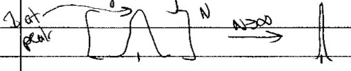
\[\begin{split}\begin{align} p_1(p_h | D_1,I) &\propto p(D_1 | p_h, I) \, p(p_h | I) \\ \\ \Longrightarrow p_2(p_h | D_1, I) &\propto p(D_1 | p_h, I) \, p_1(p_h | D_1, I) \\ &\propto [p(D_1 | p_h,I)]^2 \, p(p_h | I) \\[5pt] \mbox{What if we keep going $N$ times?}\quad & \\[5pt] \Longrightarrow p_N(p_h | D_1, I) &\propto p(D_1|p_h, I)\, p_{N-1}(p_h | D_1, I) \\ &\propto [p(D_1 | p_h, I)]^N \, p(p_h | I) \end{align}\end{split}\]Suppose \(D_1\) was 0, then \([p(\text{tails}|p_h,I)]^N \propto (1-p_h)^N p(p_h|I) \overset{N\rightarrow\infty}{\longrightarrow} \delta(p_h)\) (i.e., the posterior is only at \(p_h=0\)!). Similarly, if \(D_1\) was 1, then \([p(\text{tails}|p_h,I)]^N \propto p_h^N p(p_h|I) \overset{N\rightarrow\infty}{\longrightarrow} \delta(1-p_h)\) (i.e., the posterior is only at \(p_h=1\).)
More generally, this bootstrapping procedure would cause the posterior to get narrower and narrower with each iteration so you think you are getting more and more certain, with no new data!
Warning
Don’t do that!