7.4. Solutions

Solution to Exercise 7.1 (Correlated errors)

\[\begin{align*} \pdf{z}{I} &= \int \pdf{z}{x,y,I} \pdf{x,y}{I} dxdy = \int \delta(z-\sqrt{2}s) p(s|I) p(t|I) dsdt \\ &= \left\{ \begin{array}{l} \tilde{s}=\sqrt{2}s \, \Rightarrow \, ds = d\tilde{s}/\sqrt{2} \\ \delta(z-\sqrt{2}s) \to \delta(z/\sqrt{2}-\tilde{s}) \end{array} \right\} = \frac{1}{\sqrt{2}\sqrt{2\pi}\sigma_s}\exp \left( - \frac{z^2}{4\sigma_s^2} \right) \int p(t|I) dt . \end{align*}\]

Here we can use that \(\int p(t|I) dt = 1\). Defining \(\sigma_z = \sqrt{2}\sigma_s\) we find

\[ \pdf{z}{I} = \frac{1}{\sqrt{2\pi}\sigma_z}\exp \left( - \frac{z^2}{2\sigma_z^2} \right) , \]

i.e. a normal distribution for \(z\) with a small variance \(2\sigma_s^2\).

Solution to Exercise 7.3 (Inferring galactic distances)

1. A fixed value for \(H\) can be assigned with the PDF \(\pdf{H}{I} = \delta(H-H_0)\), where \(\delta(x)\) is the Kronecker delta. We note that integrals over a delta function are given by \(\int_{-\infty}^{+\infty} f(x) \delta(x-x_0) dx = f(x_0)\) such that

   \[ \pdf{d}{\data,I} \propto \exp\left( - \frac{(v_0 - H_0 d)^2}{2\sigma_v^2} \right), \]

   where we have ignored all normalization coefficients.

2. With a Gaussian prior for \(H\) we will be left with an integral

   \[ \pdf{d}{\data,I} \propto \int_{-\infty}^{+\infty} dH \exp\left( - \frac{(H-H_0)^2}{2 \sigma_H^2} \right) \exp\left( - \frac{(v_0 - H d)^2}{2\sigma_v^2} \right). \]

   We can perform this integral numerically, or we can solve it analytically by realizing that the product of two Gaussian distributions is another Gaussian distribution.

3. The uniform prior for \(\pdf{H}{I}\) implies that the final integral becomes

   \[ \pdf{d}{\data,I} \propto \int_{H_0 - 2\sigma_H}^{H_0 + 2\sigma_H} dH \exp\left( - \frac{(v_0 - H d)^2}{2\sigma_v^2} \right). \]

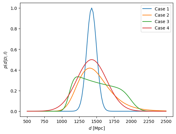
For numerical integration, and plots of the results of the three inference strategies, see the hidden code block below.

Show code cell content

Hide code cell content

# Common imports
import numpy as np
import matplotlib.pyplot as plt
import scipy.integrate as integrate

# Given information
H0=70
sigH=10
v0=10**5
sigv=5000

# grid for evaluating and plotting p(d|...)
dgrid = np.linspace(500,2500,100)

# Case 1
def pdf_1(d):
    return np.exp(-(v0-H0*d)**2/(2*sigv**2))
# Case 2
def pdf_2(H,d):
    return np.exp(-(H-H0)**2 / (2*sigH**2)) * np.exp(-(v0-H*d)**2 / (2*sigv**2))
# ... with numerical integration over H
pdf_2_grid = np.zeros_like(dgrid)
for i_d,di in enumerate(dgrid):
	I = integrate.quad(pdf_2, 0, 140, args=(di))
	pdf_2_grid[i_d] = I[0] / 20
# Case 3
def pdf_3(H,d):
    return np.exp(-(v0-H*d)**2 / (2*sigv**2))
# ... with numerical integration
pdf_3_grid = np.zeros_like(dgrid)
deltaH = np.sqrt(12*sigH**2/4)
for i_d,di in enumerate(dgrid):
	I = integrate.quad(pdf_3, H0-2*sigH, H0+2*sigH, args=(di))
	pdf_3_grid[i_d] = I[0] / 30
# Case 4 (see example 9.3)
d0 = v0/H0
sigd = d0*np.sqrt(sigH**2/H0**2 + sigv**2/v0**2)
def pdf_4(d):
    return np.exp(-(d-d0)**2 / (2*sigd**2)) / 2
    
fig,ax = plt.subplots(1,1)
ax.plot(dgrid,pdf_1(dgrid),label='Case 1')
ax.plot(dgrid,pdf_2_grid,label='Case 2')
ax.plot(dgrid,pdf_3_grid,label='Case 3')
ax.plot(dgrid,pdf_4(dgrid),label='Case 4')

ax.set_xlabel(r'$d$ [Mpc]')
ax.set_ylabel(r'$p(d|\mathcal{D},I)$')
ax.legend(loc='best');

Solution to Exercise 7.4 (The standard random variable)

The transformation \(z = f(x) = (x-\mu)/\sigma\) gives the inverse \(x = f^{-1}(z) = \sigma z + \mu\) and the Jacobian \(|dx/dz = \sigma|\).

Therefore \(\pdf{z}{I} = \pdf{x}{I} \sigma\). With the given form of \(\pdf{x}{I}\) we get

\[ \pdf{z}{I} = \frac{1}{\sqrt{2\pi}} \exp \left( -\frac{z^2}{2}\right), \]

which corresponds to a Gaussian distribution with mean zero and variance one, sometimes known as a standard random variable.

Solution to Exercise 7.5 (The square root of a number)

With \(z = f(x) = \sqrt{x}\) we have \(x = f^{-1}(z) = z^2\) such that \(|dx/dz| = 2|z|\). We note that \(z\) is positive such that \(|z| = z\) and we therefore have

\[ \pdf{z}{I} = 2 z \pdf{x}{I} = 2 z \frac{1}{x_{\max} - x_{\min}} \quad \text{for } \sqrt{x_{\min}} \leq z \leq \sqrt{x_{\max}}, \]

and 0 elsewhere.

We check the normalization by performing the integral

\[ \int_0^\infty \pdf{z}{I} dz = \int_{\sqrt{x_{\min}}}^{\sqrt{x_{\max}}} \frac{2z}{x_{\max} - x_{\min}} dz = \frac{1}{x_{\max} - x_{\min}} \left[ z^2 \right]_{\sqrt{x_{\min}}}^{\sqrt{x_{\max}}} = 1. \]

Solution to Exercise 7.6 (Gaussian sum of errors)

The PDF \(\pdf{Z}{I}\) is Gaussian with mean \(\expect{Z} = z_0 = x_0+y_0\) and variance \(\var{Z} = \sigma_z^2 = \sigma_x^2 + \sigma_y^2\), where \(x_0,y_0\) and \(\sigma_x^2, \sigma_y^2\) are the means and variances of \(X\) and \(Y\), respectively.

This is the same result as in Example 7.1 which should not be surprising since the errors were in fact Gaussian.

Solution to Exercise 7.7 (Gaussian product of errors)

The PDF \(\pdf{Z}{I}\) is Gaussian with mean \(\expect{Z} = z_0 = x_0 y_0\) and variance \(\var{Z} = \sigma_z^2 = y_0^2 \sigma_x^2 + x_0^2 \sigma_y^2\), where \(x_0,y_0\) and \(\sigma_x^2, \sigma_y^2\) are the means and variances of \(X\) and \(Y\), respectively.