📥 Demonstration: Reading Data and fitting

43.6. 📥 Demonstration: Reading Data and fitting#

Try it yourself with the Jupyter notebook

Note that demonstration sections such as this one correspond to a Jupyter Notebook that you can run yourself (rather than just looking at the static version shown here). You are highly encouraged to download the source files of the lecture notes such that you have local access to these notebooks.

Our first data set is going to be a classic from nuclear physics, namely all available data on binding energies. Don’t be intimidated if you are not familiar with nuclear physics. It serves simply as an example here of a data set.

We will show some of the strengths of packages like Scikit-Learn in fitting nuclear binding energies to specific functions using linear regression. First, however, we need to meet the Pandas.

# For showing plots inline
%matplotlib inline

Meet the Pandas#

Pandas is a very useful Python package for reading and organizing data. It is an open source library providing high-performance, easy-to-use data structures and data analysis tools for Python.

pandas stands for panel data, a term borrowed from econometrics and is an efficient library for data analysis with an emphasis on tabular data. pandas has two major classes, the DataFrame class with two-dimensional data objects such as tabular data organized in columns, and the class Series with a focus on one-dimensional data objects. Both classes allow you to index data easily as we will see in the examples below. pandas allows you also to perform mathematical operations on the data, spanning from simple reshaping of vectors and matrices to statistical operations.

The following simple example shows how we can make tables of our data. Here we define a data set which includes names, place of birth and date of birth, and displays the data in an easy to read way.

import pandas as pd
from IPython.display import display
data = {'First Name': ["Frodo", "Bilbo", "Aragorn II", "Samwise"],
        'Last Name': ["Baggins", "Baggins","Elessar","Gamgee"],
        'Place of birth': ["Shire", "Shire", "Eriador", "Shire"],
        'Date of Birth T.A.': [2968, 2890, 2931, 2980]
        }
data_pandas = pd.DataFrame(data)
display(data_pandas)

	First Name	Last Name	Place of birth	Date of Birth T.A.
0	Frodo	Baggins	Shire	2968
1	Bilbo	Baggins	Shire	2890
2	Aragorn II	Elessar	Eriador	2931
3	Samwise	Gamgee	Shire	2980

In the above example we have imported pandas with the shorthand pd, the latter has become the standard way to import pandas. We then make a dictionary with various variables and reorganize the lists of values into a DataFrame and then print out a neat table with specific column labels as Name, place of birth and date of birth. Displaying these results, we see that the indices are given by the default numbers from zero to three. pandas is extremely flexible and we can easily change the above indices by defining a new type of indexing as

data_pandas = pd.DataFrame(data,index=['Frodo','Bilbo','Aragorn','Sam'])
display(data_pandas)

	First Name	Last Name	Place of birth	Date of Birth T.A.
Frodo	Frodo	Baggins	Shire	2968
Bilbo	Bilbo	Baggins	Shire	2890
Aragorn	Aragorn II	Elessar	Eriador	2931
Sam	Samwise	Gamgee	Shire	2980

Thereafter we display the content of the row which begins with the index Aragorn

display(data_pandas.loc['Aragorn'])

First Name            Aragorn II
Last Name                Elessar
Place of birth           Eriador
Date of Birth T.A.          2931
Name: Aragorn, dtype: object

We can easily append data to this DataFrame, for example using concat (note that the function append was deprecated in pandas 2.0)

new_hobbit = {'First Name': ["Peregrin"],
              'Last Name': ["Took"],
              'Place of birth': ["Shire"],
              'Date of Birth T.A.': [2990]
              }
data_pandas=pd.concat([data_pandas,pd.DataFrame(new_hobbit, index=['Pippin'])])
display(data_pandas)

	First Name	Last Name	Place of birth	Date of Birth T.A.
Frodo	Frodo	Baggins	Shire	2968
Bilbo	Bilbo	Baggins	Shire	2890
Aragorn	Aragorn II	Elessar	Eriador	2931
Sam	Samwise	Gamgee	Shire	2980
Pippin	Peregrin	Took	Shire	2990

Here are other examples where we use the DataFrame functionality to handle arrays, now with more interesting features for us, namely numbers. We set up a matrix of dimensionality \(10\times 5\) and compute the mean value and standard deviation of each column. Similarly, we can perform mathematical operations like squaring the matrix elements and many other operations.

import numpy as np
import pandas as pd
from IPython.display import display
np.random.seed(100)
# setting up a 10 x 5 matrix
rows = 10
cols = 5
a = np.random.randn(rows,cols)
df = pd.DataFrame(a)
display(df)
print(df.mean())
print(df.std())
display(df**2)

	0	1	2	3	4
0	-1.749765	0.342680	1.153036	-0.252436	0.981321
1	0.514219	0.221180	-1.070043	-0.189496	0.255001
2	-0.458027	0.435163	-0.583595	0.816847	0.672721
3	-0.104411	-0.531280	1.029733	-0.438136	-1.118318
4	1.618982	1.541605	-0.251879	-0.842436	0.184519
5	0.937082	0.731000	1.361556	-0.326238	0.055676
6	0.222400	-1.443217	-0.756352	0.816454	0.750445
7	-0.455947	1.189622	-1.690617	-1.356399	-1.232435
8	-0.544439	-0.668172	0.007315	-0.612939	1.299748
9	-1.733096	-0.983310	0.357508	-1.613579	1.470714

 -0.175300
  0.083527
 -0.044334
 -0.399836
  0.331939
dtype: float64
  1.069584
  0.965548
  1.018232
  0.793167
  0.918992
dtype: float64

	0	1	2	3	4
0	3.061679	0.117430	1.329492	0.063724	0.962990
1	0.264421	0.048920	1.144993	0.035909	0.065026
2	0.209789	0.189367	0.340583	0.667239	0.452553
3	0.010902	0.282259	1.060349	0.191963	1.250636
4	2.621102	2.376547	0.063443	0.709698	0.034047
5	0.878123	0.534362	1.853835	0.106431	0.003100
6	0.049462	2.082875	0.572069	0.666597	0.563167
7	0.207888	1.415201	2.858185	1.839818	1.518895
8	0.296414	0.446453	0.000054	0.375694	1.689345
9	3.003620	0.966899	0.127812	2.603636	2.162999

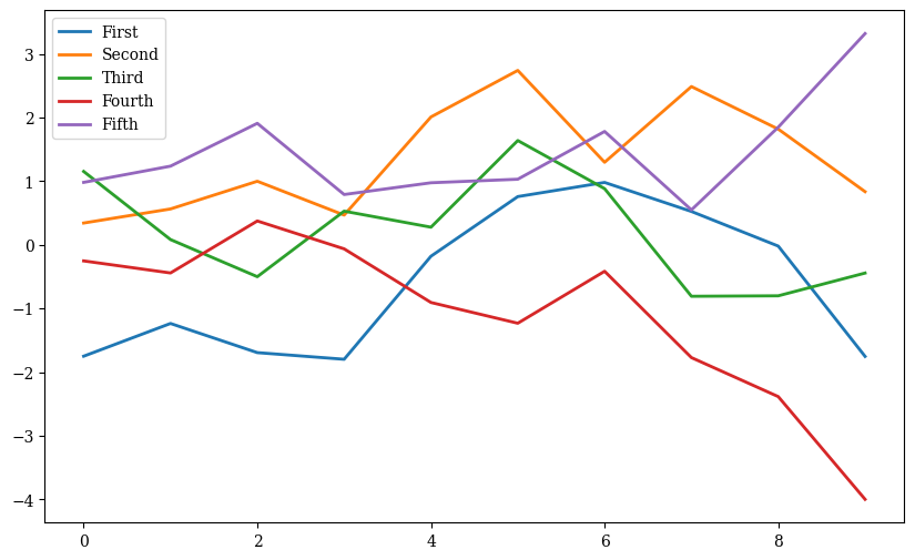
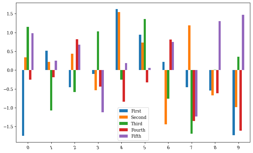
Thereafter we can select specific columns only and plot final results

df.columns = ['First', 'Second', 'Third', 'Fourth', 'Fifth']
df.index = np.arange(10)

display(df)
print(df['Second'].mean() )
print(df.info())
print(df.describe())

from pylab import plt, mpl
mpl.rcParams['font.family'] = 'serif'

df.cumsum().plot(lw=2.0, figsize=(10,6));

df.plot.bar(figsize=(10,6), rot=15);

	First	Second	Third	Fourth	Fifth
0	-1.749765	0.342680	1.153036	-0.252436	0.981321
1	0.514219	0.221180	-1.070043	-0.189496	0.255001
2	-0.458027	0.435163	-0.583595	0.816847	0.672721
3	-0.104411	-0.531280	1.029733	-0.438136	-1.118318
4	1.618982	1.541605	-0.251879	-0.842436	0.184519
5	0.937082	0.731000	1.361556	-0.326238	0.055676
6	0.222400	-1.443217	-0.756352	0.816454	0.750445
7	-0.455947	1.189622	-1.690617	-1.356399	-1.232435
8	-0.544439	-0.668172	0.007315	-0.612939	1.299748
9	-1.733096	-0.983310	0.357508	-1.613579	1.470714

0.08352721390288316
<class 'pandas.core.frame.DataFrame'>
Index: 10 entries, 0 to 9
Data columns (total 5 columns):
 #   Column  Non-Null Count  Dtype  
---  ------  --------------  -----  
 0   First   10 non-null     float64
 1   Second  10 non-null     float64
 2   Third   10 non-null     float64
 3   Fourth  10 non-null     float64
 4   Fifth   10 non-null     float64
dtypes: float64(5)
memory usage: 480.0 bytes
None
           First     Second      Third     Fourth      Fifth
count  10.000000  10.000000  10.000000  10.000000  10.000000
mean   -0.175300   0.083527  -0.044334  -0.399836   0.331939
std     1.069584   0.965548   1.018232   0.793167   0.918992
min    -1.749765  -1.443217  -1.690617  -1.613579  -1.232435
25%    -0.522836  -0.633949  -0.713163  -0.785061   0.087887
50%    -0.280179   0.281930  -0.122282  -0.382187   0.463861
75%     0.441264   0.657041   0.861676  -0.205231   0.923602
max     1.618982   1.541605   1.361556   0.816847   1.470714

../../_images/19a59f59f042ed9e3edf4c517b12bcc7f72b464319929d374baa061284d73679.png

../../_images/ffcd426d5108e23b2156f4460c436b9adf434c758a095618709e9d79e06511ae.png

We can produce a \(4\times 4\) matrix

b = np.arange(16).reshape((4,4))
print(b)
df1 = pd.DataFrame(b)
print(df1)

[[ 0  1  2  3]
 [ 4  5  6  7]
 [ 8  9 10 11]
 [12 13 14 15]]
    0   1   2   3
0   0   1   2   3
1   4   5   6   7
2   8   9  10  11
3  12  13  14  15

and many other operations.

The Series class is another important class included in pandas. You can view it as a specialization of DataFrame but where we have just a single column of data. It shares many of the same features as DataFrame. As with DataFrame, most operations are vectorized, achieving thereby a high performance when dealing with computations of arrays, in particular labeled arrays. As we will see below it leads also to a very concice code close to the mathematical operations we may be interested in. For multidimensional arrays, we recommend strongly xarray. xarray has much of the same flexibility as pandas, but allows for the extension to higher dimensions than two.

To our real data: nuclear binding energies. Brief reminder on masses and binding energies#

Let us now dive into nuclear physics and remind ourselves briefly about some basic features about binding energies. A basic quantity which can be measured for the ground states of nuclei is the atomic mass \(M(N, Z)\) of the neutral atom with atomic mass number \(A\) and charge \(Z\). The number of neutrons is \(N\). There are indeed several sophisticated experiments worldwide which allow us to measure this quantity to high precision (parts per million even).

Atomic masses are usually tabulated in terms of the mass excess defined by

\[ \Delta M(N, Z) = M(N, Z) - uA, \]

where \(u\) is the Atomic Mass Unit

\[ u = M(^{12}\mathrm{C})/12 = 931.4940954(57) \hspace{0.1cm} \mathrm{MeV}/c^2. \]

The nucleon masses are

\[ m_p = 1.00727646693(9)u, \]

and

\[ m_n = 939.56536(8)\hspace{0.1cm} \mathrm{MeV}/c^2 = 1.0086649156(6)u. \]

In the 2016 mass evaluation of by W.J.Huang, G.Audi, M.Wang, F.G.Kondev, S.Naimi and X.Xu [WAK+17] there are data on masses and decays of 3437 nuclei.

The nuclear binding energy is defined as the energy required to break up a given nucleus into its constituent parts of \(N\) neutrons and \(Z\) protons. In terms of the atomic masses \(M(N, Z)\) the binding energy is defined by

\[ BE(N, Z) = ZM_H c^2 + Nm_n c^2 - M(N, Z)c^2 , \]

where \(M_H\) is the mass of the hydrogen atom and \(m_n\) is the mass of the neutron. In terms of the mass excess the binding energy is given by

\[ BE(N, Z) = Z\Delta_H c^2 + N\Delta_n c^2 -\Delta(N, Z)c^2 , \]

where \(\Delta_H c^2 = 7.2890\) MeV and \(\Delta_n c^2 = 8.0713\) MeV.

A popular and physically intuitive model which can be used to parametrize the experimental binding energies as function of \(A\), is the so-called liquid drop model. The ansatz is based on the following expression

\[ BE(N,Z) = a_1A-a_2A^{2/3}-a_3\frac{Z(Z-1)}{A^{1/3}}-a_4\frac{(N-Z)^2}{A}, \]

where \(A\) stands for the number of nucleons and the \(a_i\)s are parameters which are determined by a fit to the experimental data.

To arrive at the above expression we have assumed that we can make the following assumptions:

There is a volume term \(a_1A\) proportional to the number of nucleons. When an assembly of nucleons of the same size is packed together into the smallest volume, each interior nucleon has a certain number of other nucleons in contact with it. This contribution is proportional to the volume. Note that the nuclear radius is empirically proportional to \(A^{1/3}\).

There is a surface energy term \(a_2A^{2/3}\). The assumption here is that a nucleon at the surface of a nucleus interacts with fewer other nucleons than one in the interior of the nucleus and hence its binding energy is less. This surface energy term takes that into account and is therefore negative and is proportional to the surface area.

There is a Coulomb energy term \(a_3\frac{Z(Z-1)}{A^{1/3}}\). The electric repulsion between each pair of protons in a nucleus yields less binding.

There is an asymmetry term \(a_4\frac{(N-Z)^2}{A}\). This term is associated with the Pauli exclusion principle and reflects the fact that the proton-neutron interaction is more attractive on the average than the neutron-neutron and proton-proton interactions.

We could also add a so-called pairing term, which is a correction term that arises from the tendency of proton pairs and neutron pairs to occur. An even number of particles is more stable than an odd number.

Import modules#

We import also various modules that we will find useful in order to present various Machine Learning methods. Here we focus mainly on the functionality of scikit-learn.

%matplotlib inline

# Common imports
import numpy as np
import pandas as pd
import matplotlib.pyplot as plt
import sklearn.linear_model as skl
from sklearn.model_selection import train_test_split
from sklearn.metrics import mean_squared_error, r2_score, mean_absolute_error
import os

# Nicer plots
import seaborn as sns
sns.set('talk')

Organizing our data#

Let us start with reading and organizing our data. We start with the compilation of masses and binding energies from 2016. After having downloaded this file to our own computer, we are now ready to read the file and start structuring our data.

We start with preparing folders for storing our calculations and the data file over masses and binding energies.

# Where to save the figures and data files
PROJECT_ROOT_DIR = "Results"
FIGURE_ID = "Results/FigureFiles"
DATA_ID = "DataFiles/"

if not os.path.exists(PROJECT_ROOT_DIR):
    os.mkdir(PROJECT_ROOT_DIR)

if not os.path.exists(FIGURE_ID):
    os.makedirs(FIGURE_ID)

if not os.path.exists(DATA_ID):
    os.makedirs(DATA_ID)

def image_path(fig_id):
    return os.path.join(FIGURE_ID, fig_id)

def data_path(dat_id):
    return os.path.join(DATA_ID, dat_id)

def save_fig(fig_id):
    plt.savefig(image_path(fig_id) + ".png", format='png')

Our next step is to read the data on experimental binding energies and reorganize them as functions of the mass number \(A\), the number of protons \(Z\) and neutrons \(N\) using pandas. Before we do this it is always useful (unless you have a binary file or other types of compressed data) to actually open the file and simply take a look at it!

Note: In the cell below, infile is an iterator and after you show the first 42 lines, the iterator will point to the 43rd line. In order to avoid reading the file from a non-expected start point, we put the iteration and print commands within a with block which means that infile is only defined inside this block and will then be forgotten. Thanks to (@Daniel Berg} for finding this bug.

with open(data_path("MassEval2016.dat"),'r') as infile:
    head = [next(infile) for x in np.arange(42)]
    print("".join(head))

1    a0boogfu                                 A T O M I C   M A S S   A D J U S T M E N T
0                                                     DATE  1 Mar 2017 TIME 17:26
0        *********************                               A=   0 TO 295
         * file : mass16.txt *
         *********************

   This is one file out of a series of 3 files published in:
       "The Ame2016 atomic mass evaluation (I)"   by W.J.Huang, G.Audi, M.Wang, F.G.Kondev, S.Naimi and X.Xu
           Chinese Physics C41 030002, March 2017.
       "The Ame2016 atomic mass evaluation (II)"  by M.Wang, G.Audi, F.G.Kondev, W.J.Huang, S.Naimi and X.Xu
           Chinese Physics C41 030003, March 2017.
                       for files : mass16.txt  : atomic masses
                                   rct1-16.txt : react and sep energies,  part 1
                                   rct2-16.txt : react and sep energies,  part 2
   A fourth file  is the "Rounded" version of the atomic mass table (the first file)
                                   mass16round.txt : atomic masses "Rounded" version

   All files are 3436 lines long with 124 character per line.
       Headers are 39 lines long.
   Values in files 1, 2 and 3 are unrounded copy of the published ones
   Values in file  4          are exact     copy of the published ones

   col 1     :  Fortran character control: 1 = page feed  0 = line feed
   format    :  a1,i3,i5,i5,i5,1x,a3,a4,1x,f13.5,f11.5,f11.3,f9.3,1x,a2,f11.3,f9.3,1x,i3,1x,f12.5,f11.5
                cc NZ  N  Z  A    el  o     mass  unc binding unc     B  beta  unc    atomic_mass   unc
   Warnings  :  this format is identical to the ones used in Ame2003 and Ame2012
                      in particular "Mass Excess" and "Atomic Mass" values are given now, when necessary,
                      with 5 digits after decimal point.
                decimal point is replaced by # for (non-experimental) estimated values.
                * in place of value : not calculable

....+....1....+....2....+....3....+....4....+....5....+....6....+....7....+....8....+....9....+...10....+...11....+...12....


                                                               MASS LIST
                                                             for analysis

1N-Z    N    Z   A  EL    O     MASS EXCESS       BINDING ENERGY/A        BETA-DECAY ENERGY         ATOMIC MASS
                                   (keV)                (keV)                    (keV)                (micro-u)
0  1    1    0    1  n         8071.31713    0.00046      0.0      0.0   B-    782.347    0.000   1 008664.91582    0.00049
  -1    0    1    1 H          7288.97061    0.00009      0.0      0.0   B-      *                1 007825.03224    0.00009
0  0    1    1    2 H         13135.72176    0.00011   1112.283    0.000 B-      *                2 014101.77811    0.00012

In particular, the program that outputs the final nuclear masses is written in Fortran with a specific format. It means that we need to figure out the format and which columns contain the data we are interested in. Pandas comes with a function that reads formatted output. After having admired the file, we are now ready to start massaging it with pandas.

The file begins with some basic format information in the header (that is 39 lines long).
The data we are interested in are in columns 2, 3, 4 and 11, giving us the number of neutrons, protons, mass numbers and binding energies, respectively.
We add also for the sake of completeness the element name.
The data are in fixed-width formatted lines and we will convert them into the pandas DataFrame structure.
The liquid drop model does not work well for the lightest elements so we skip the first few lines of data in the file (we could as well have made this cut after actually reading the data).
The data is for the binding energy per nucleon (not the total binding energy as in the formula). We will need to be careful to compare the same quantities.

# Open the file again and read the experimental data with Pandas
with open(data_path("MassEval2016.dat"),'r') as infile:
    Masses = pd.read_fwf(infile, usecols=(2,3,4,6,11),
              names=('N', 'Z', 'A', 'Element', 'Ebinding'),
              widths=(1,3,5,5,5,1,3,4,1,13,11,11,9,1,2,11,9,1,3,1,12,11,1),
              header=64,
              index_col=False)

# Extrapolated values are indicated by '#' in place of the decimal place, so
# the Ebinding column won't be numeric. Coerce to float and drop these entries.
Masses['Ebinding'] = pd.to_numeric(Masses['Ebinding'], errors='coerce')
Masses = Masses.dropna()
# Convert from keV to MeV.
Masses['Ebinding'] /= 1000

# Group the DataFrame by nucleon number, A.
Masses = Masses.groupby('A')
# Find the rows of the grouped DataFrame with the maximum binding energy.
Masses = Masses.apply(lambda t: t[t.Ebinding==t.Ebinding.max()])

/tmp/ipykernel_7186/3733791492.py:19: FutureWarning: DataFrameGroupBy.apply operated on the grouping columns. This behavior is deprecated, and in a future version of pandas the grouping columns will be excluded from the operation. Either pass `include_groups=False` to exclude the groupings or explicitly select the grouping columns after groupby to silence this warning.
  Masses = Masses.apply(lambda t: t[t.Ebinding==t.Ebinding.max()])

We have now read in the data, grouped them according to the variables we are interested in. We see how easy it is to reorganize the data using pandas. If we were to do these operations in C/C++ or Fortran, we would have had to write various functions/subroutines which perform the above reorganizations for us. Having reorganized the data, we can now start to make some simple fits using both the functionalities in numpy and Scikit-Learn afterwards.

Now we define five variables which contain the number of nucleons \(A\), the number of protons \(Z\) and the number of neutrons \(N\), the element name and finally the energies themselves.

A = Masses['A']
Z = Masses['Z']
N = Masses['N']
Element = Masses['Element']
TotalEnergies = Masses['Ebinding'] * Masses['A']
print(Masses)

            N    Z    A Element  Ebinding
A                                        
2       6    4   10      Be  6.497630
8       6    5   11       B  6.927732
14      6    6   12       C  7.680144
20      7    6   13       C  7.469849
25      8    6   14       C  7.520319
...       ...  ...  ...     ...       ...
3272  156  108  264      Hs  7.298375
3278  157  108  265      Hs  7.296247
3285  158  108  266      Hs  7.298273
3306  159  110  269      Ds  7.250154
3312  160  110  270      Ds  7.253775

[258 rows x 5 columns]

The next step, and we will define this mathematically later, is to set up the so-called design matrix. We will throughout call this matrix \(\boldsymbol{X}\). It has dimensionality \(n\times p\), where \(n\) is the number of data points and \(p\) are the so-called predictors or features. In our case they are given by the functions of \(A\) (and \(N\), \(Z\)) that are included in the liquid drop model and that we wish to include in the fit.

We will make the fit with respect to the total binding energy. One could argue that it would be better to fit to the binding energy per nucleon. Can you argue why that is?

Note that we also include a constant term (an intercept) since this is expected by the LinearRegression method that we will be using.

# Now we set up the design matrix X
X = np.zeros((len(A),5))
X[:,0] = np.ones_like(A)
X[:,1] = A
X[:,2] = A**(2.0/3.0)
X[:,3] = Z*(Z-1) * A**(-1.0/3.0)
X[:,4] = (N-Z)**2 * A**(-1.0)

With scikitlearn we are now ready to use linear regression and fit our data. Note that we have included an intercept column into our design matrix, which corresponds to a constant predictor term in our model. It is very common to have such a term in a linear regression fit and we include it here although our model actually does not have such a predictor. In fact, the built-in linear regression function that we will use does usually add such an offset automatically and we need to explicitly turn it off using the argument fit_intercept=False since we already have it in our design matrix.

clf = skl.LinearRegression(fit_intercept=False).fit(X, TotalEnergies)
fity = clf.predict(X)

Pretty simple! Now we can print measures of how our fit is doing, the coefficients from the fits and plot the final fit together with our data.

# The mean squared error                               
print(f"Mean squared error (for energy per nucleon): {mean_squared_error(TotalEnergies/A, fity/A):.3f}")
# Explained variance score: 1 is perfect prediction                                 
print(f'Variance score (for energy per nucleon): {r2_score(TotalEnergies/A, fity/A):.3f}')
# Mean absolute error                                                           
print(f'Mean absolute error (for energy per nucleon): {mean_absolute_error(TotalEnergies/A, fity/A):.3f}')

Mean squared error (for energy per nucleon): 0.002
Variance score (for energy per nucleon): 0.990
Mean absolute error (for energy per nucleon): 0.025

print(clf.coef_)
# Or nicer
print('***')
print('intercept  volume    surface    coulomb     asymmetry')
print("     ".join(["%.3f"%coef for coef in clf.coef_]))

[ 19.06802716  17.20433313 -24.05418781  -0.78693299 -26.3490481 ]
***
intercept  volume    surface    coulomb     asymmetry
19.068     17.204     -24.054     -0.787     -26.349

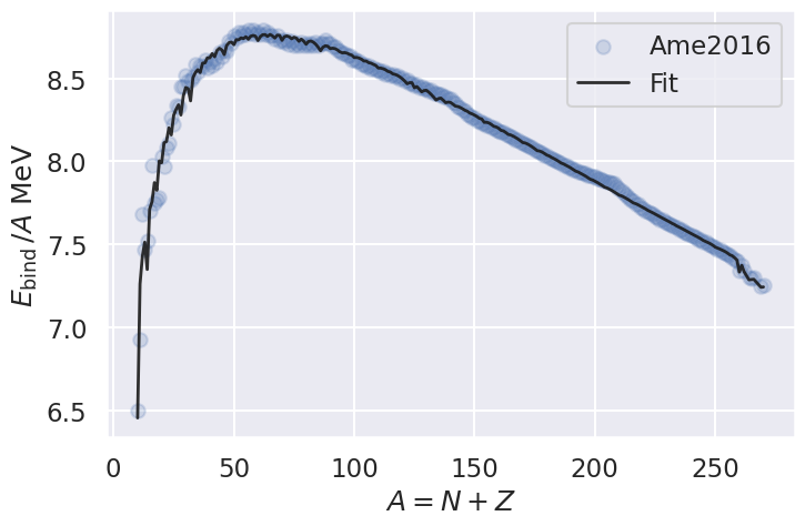
# Generate a plot comparing the experimental with the fitted values values.
Masses['Eapprox']  = fity/A
fig, ax = plt.subplots(figsize=(8,5))
ax.set_xlabel(r'$A = N + Z$')
ax.set_ylabel(r'$E_\mathrm{bind}\,/A$ MeV')
ax.scatter(Masses['A'], Masses['Ebinding'], alpha=0.2, marker='o',
            label='Ame2016')
ax.plot(Masses['A'], Masses['Eapprox'], alpha=0.9, lw=2, c='k',
            label='Fit')
ax.legend()
save_fig("Masses2016")

../../_images/60e5ec24d37c6a3f732b4e3c47a4621e77c06ec5f86a0031a9e9878357163913.png

A first summary#

The aim behind these introductory words was to present to you various Python libraries and their functionalities, in particular libraries like numpy, pandas, and matplotlib and other that make our life much easier in handling various data sets and visualizing data.

Furthermore, Scikit-Learn allows us with few lines of code to implement popular Machine Learning algorithms for supervised learning.

A physics remark that concerns the liquid drop model for nuclear binding energies is that we fail to reproduce some slow variations in the target data. In fact, we know that these variations are due to shell effects, with local maxima appearing in binding energies as different shells and subshells are filled.