11.2. Framework

We begin by setting up the model discrepancy framework following KOH. Let the \(i\)-th measurement for an observable \(y\) be denoted as

(11.2)\[ y(x_i) \sim \zeta(x_i) + \epsilon_i \,, \qquad \epsilon_i \sim \mathcal{N}(0,\sigma_i^2) \,. \]

Here, the index \(i\) corresponds to the point in input space \(x\) where the \(i\)-th observation is made (e.g., a specific time in the ball drop experiment described below). Independent observation errors \(\epsilon_i\) are assumed to follow Gaussian distributions with zero mean and standard deviation \(\sigma_i\). Here, \(\zeta(x_i)\) represents the true value of the observable at \(x_i\). (We assume that \(x\) is made unitless by scaling it with a suitable reference scale \(x_0\).)

We denote the prediction from a theoretical model for the observable \(y\) as \(\eta(x, \pars)\), where \(\pars\) is the vector of true but unknown model parameters. The model for \(\eta(x,\pars)\) is then defined as:

(11.3)\[ \zeta(x) = \eta(x, \pars) + \delta(x) ; \]

here \(\delta(x)\) quantifies the discrepancy between the theoretical model prediction and the true system value at input setting \(x\). Combining the above equations, we express the observation \(y(x_i)\) as

(11.4)\[ y(x_i) \sim \eta(x_i, \pars) + \delta(x_i) + \epsilon_i . \]

Thus, each observation is modeled as the sum of the model output (evaluated at the true \(\pars\)), the model discrepancy \(\delta\) at \(x_i\), and the observational error \(\epsilon_i\). The statiscal model is summarized in Fig. 11.1.

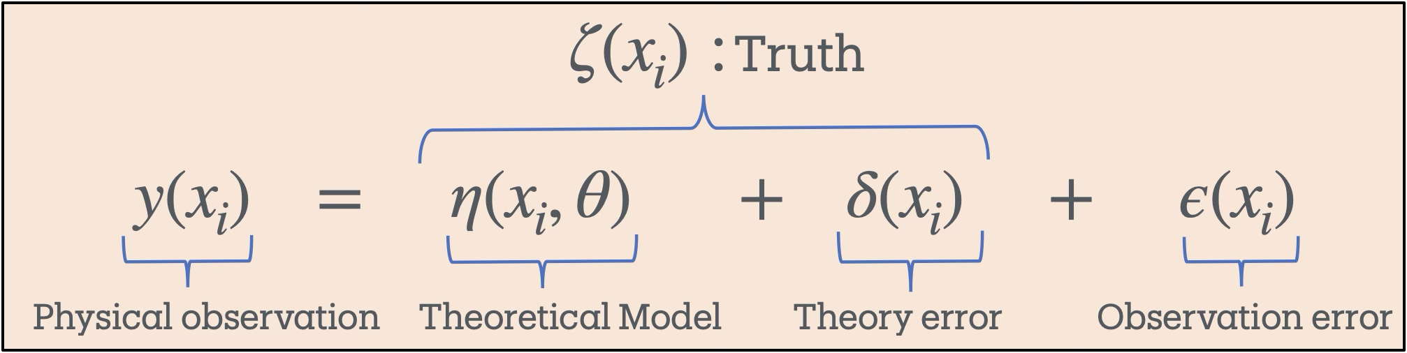
Fig. 11.1 Statistical model.

Following KOH, we represent \(\delta(x)\) as a zero-mean Gaussian process (GP):

\[ \delta(\cdot \mid\boldsymbol{\phi}) \sim {\rm GP} \left(\boldsymbol{0}, K(\cdot,\cdot \mid\boldsymbol{\phi}) \right) \,, \]

where \(K(\cdot,\cdot \mid\boldsymbol{\phi})\) is the covariance kernel, which depends on a set of hyperparameters \(\boldsymbol{\phi}\). A GP specifies a distribution over functions, with the covariance kernel \(K\) serving as the central object that defines the properties of the functions in the distribution. In this framework, we incorporate prior knowledge about the theoretical model’s uncertainties through the choice of the covariance kernel. Adopting a Bayesian approach, we assign prior probability distributions to both the model parameters \(\pars\) and the GP hyperparameters \(\boldsymbol{\phi}\), and update these to obtain their posterior distributions conditioned on the observations. In all examples discussed in this work, uniform priors (in appropriate ranges) are used for both the model parameters and the GP hyperparameters.

The particular \(K\) we use for the test case explored here is

(11.5)\[ K(x_i, x_j) = {\color{ForestGreen}{\bar{c}}}^2 (x_i x_j)^{\color{ForestGreen}{r}} \exp\left(- \frac{\lVert x_i-x_j\rVert^2}{2{\color{ForestGreen}{\ell}}^2} \right) \]

The hyperparameters control the nature of the possible random draws, as illustrated in Fig. 11.2. The parameter \(\bar{c}\), which is fixed at \(\bar{c}=1\) in the figure, controls the overall scale over which the random functions vary. The parameter \(\ell\) is the correlation length between any two points; as \(|x -x'|\) becomes greater than \(\ell\), the points become increasingly uncorrelated. Comparing \(\ell=1\) to \(\ell=3\) shows that the latter curves have a longer “wavelength”. Finally, \(r\) is a parameter introduced to generate functions that increase with \(x\) for \(r>0\).

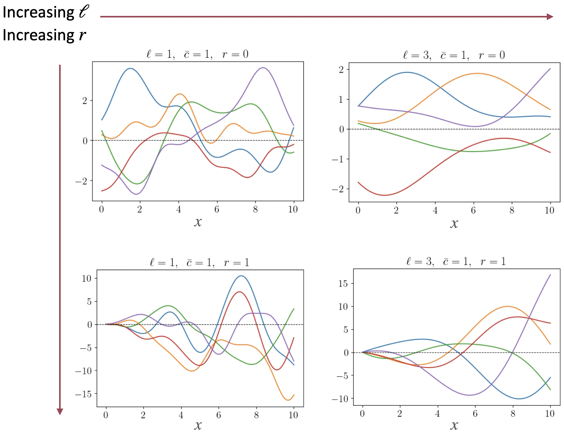
Fig. 11.2 Five draws from each of four GPs of the form in Eq. (11.5) with hyperparameters \(\ell\), \(\bar c\), and \(r\) as listed.

Note

If sampled at any one input point \(x\), the prior GP will yield a Gaussian distribution with mean and variance specified by the GP definition. In many cases, the prior GP is taken to be mean zero with a constant variance for all \(x\). If sampled at any two input points \(x\) and \(x'\), the joint distribution will be a bivariate Gaussian, with covariance given by \(K(x,x'|\boldsymbol{\phi})\).