8.2. Bayesian research workflow

In Bayesian workflow we presented a four-step Bayesian workflow, repeated here:

Four-step Bayesian workflow in brief

1. Formulate informative priors before new data is used.

2. Define a statistical model relating the physics model and data, including all errors.

3. Compute the posterior probabilities.

4. Do model checking.

In this chapter we elaborate on these steps. We start with a condensed description of a Bayesian workflow for rigorous scientific inference. It is based on the more extensive exposition in the Methods Primer by Van De Schoot et al. [vandSchootDK+21].

This formulation divides a typical Bayesian workflow into three main steps (see Fig. 8.7): (i) capturing available knowledge about given parameters in a statistical model via the prior distribution (typically performed before data collection); (ii) determining the likelihood function using the information about the data generating process; and (iii) combining both the prior distribution and the likelihood function using Bayes’ theorem in the form of the posterior distribution. The posterior distribution is used to conduct inferences. These steps correspond to those we have introduced, except that step 4 is not made explicit. In the following subsections we expand upon each step.

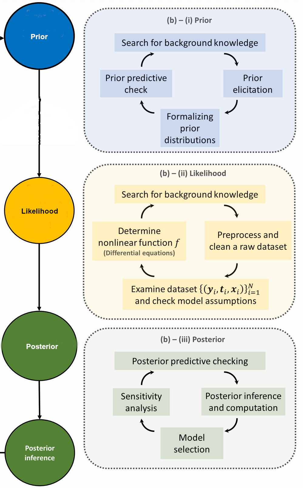
Fig. 8.7 The Bayesian research cycle. The steps needed for a research cycle using Bayesian statistics include formalizing prior distributions based on background knowledge and prior elicitation; determining the likelihood function by specifying a data-generating model and including observed data; and obtaining the posterior distribution as a function of both the specified prior and the likelihood function. After obtaining the posterior results, inferences can be made that can then be used to start a new research cycle. Attribution: Stat math, CC BY-SA 4.0, via Wikimedia Commons. See also [vandSchootDK+21].

Experimentation (of the statistical model)

The first two steps in the Bayesian workflow described in Fig. 8.7) are key to a rigorous inference process and are sometimes known as the (statistical) experimentation phase. Prior distributions, shortened to priors, are first determined. The selection of priors is often viewed as one of the more important choices that a researcher makes when implementing a Bayesian model as it can have a substantial impact on the final results. The appropriateness of the priors being implemented is ascertained using a prior predictive checking process (see Remark 8.1). The likelihood function, shortened to likelihood, is then determined. Given the important roles that the prior and the likelihood have in determining the posterior, it is imperative that these steps are conducted with care.

Formalizing prior distributions

Priors can come in many different distributional forms, such as a normal, uniform or Poisson distribution, among others. Most importantly, priors can have different levels of informativeness. The information reflected in a prior distribution can be anywhere on a continuum from complete uncertainty to relative certainty. Although priors can fall anywhere along this continuum, there are three main classifications of priors that are used in the literature to categorize the degree of (un)certainty surrounding the parameter value: informative, weakly informative and diffuse. These classifications can be made based on the researcher’s personal judgement. For example, the variance (or width) of a normal distribution is linked to its level of informativeness. A variance of 1,000 may be considered diffuse in one research setting and informative in another, depending on the likelihood function as well as the scaling for the parameter. A good practical guide to choosing priors is the Stan Prior Choice Recommendations on github.

Prior elicitation.

Prior elicitation is the process by which a suitable prior distribution is constructed. Strategies for prior elicitation include asking an expert or a panel of experts to provide values for the hyperparameters of the prior distribution.

Prior elicitation can also involve implementing data-based priors. Then, the hyperparameters for the prior are derived from sample data using methods such as maximum likelihood. Such approaches, however, risk leading to double-dipping, as the same sample data set might be used to derive prior distributions and to obtain the posterior. Double-dipping must be avoided in a rigorous analysis.

The subjectivity of priors is highlighted by critics as a potential drawback of Bayesian methods. Two distinct points should be mentioned in this context. First, many elements of the estimation process are subjective, aside from prior selection, including the model itself and the error assumptions. To place the notion of subjectivity solely on the priors is a misleading distraction from the other elements in the process that are inherently subjective. Second, priors are not necessarily a point of subjectivity. For example, there are circumstances when informative priors are needed.

Priors are typically defined through previous beliefs, information or knowledge. Although beliefs can be characterized as subjective points of view from the researcher, information is typically quantifiable, and knowledge can be defined as objective and consensus-based.

Sometimes, diffuse priors are assigned to reflect an indifference to the location or scale of some parameter. Symmetry arguments can then be used to assign a prior that reflects this indifference of symmetry invariance. See Section 12.1 for more on this topic and specific examples.

Even with quantified prior information, the choice of distributional form for the prior (as needed for a full Bayesian analysis) typically involves extra assumptions. Say that you wish to assign a prior with a specific mean value and standard deviation for a model parameter. In this scenario you are still left with the choice between many different distributional forms that fulfil those constraints. Fortunately, arguments based on the maximum entropy principle can help translating a finite set of prior knowledge into a probability distribution with the least restrictive extra assumptions. These ideas are presented in Section 12.2 Assigning probabilities (II): The principle of maximum entropy.

Because inference based on a Bayesian analysis is subject to the “correctness” of the prior, it is of importance to carefully check whether the specified model can be considered to be generating the actual data. This is partly done by means of a process known as prior predictive checking (see box below).

The prior predictive distribution is a distribution of all possible data that could be sampled if the statistical model is true. In theory, a ‘correct’ prior provides a prior predictive distribution similar to the true data-generating distribution. Prior predictive checking compares the observed data, or statistics of the observed data, with the prior predictive distribution, or statistics of the predictive distribution, and checks their compatibility.

Determining the likelihood function

The likelihood is used in both Bayesian and frequentist inference. In both inference paradigms, its role is to quantify the strength of support the observed data lends to possible value(s) for the unknown parameter(s). The key difference between Bayesian and frequentist inference is that frequentists do not consider probability statements about the unknown parameters to be useful. Instead, the unknown parameters are considered to be fixed; the likelihood is the conditional probability distribution \(\pdf{\output}{\para}\) of the data (\(\output\)), given fixed parameters (\(\para\)). In Bayesian inference, unknown parameters are referred to as random variables in order to make probability statements about them. The (observed) data are treated as fixed, whereas the parameter values are varied; the likelihood is a function of \(\para\) for the fixed data \(\output\). Therefore, the likelihood function summarizes the following elements: a statistical model that stochastically generates all of the data, a range of possible values for \(\para\) and the observed data \(\output\).

The statistical model should also account for possible correlations in both the input parameters (known as type x correlations) or in the outputs (type y). The former usually enter the prior and the latter in the likelihood. Both of them result in multivariate statistical distributions that do not simply factor into a product of independent, univariate ones.

In some cases, specifying a likelihood function can be very straightforward. However, in practice, the underlying data-generating model is not always known. Researchers often naively choose a certain data-generating model out of habit or because they cannot easily change it in the software. Although based on background knowledge, the choice of the statistical data-generating model is subjective and should therefore be well understood, clearly documented and available to the reader. Robustness checks should be performed on the selected likelihood function to verify its influence on the posterior estimates.

The sensitivity of the posterior to the inclusion of different output in the likelihood is reflective of the information content of that observable. Sensitivity studies of the posterior based on simulated outputs for different future data is a branch of statistical inference known as experimental design. It can help determine which observable(s) to spend resources on measuring to improve the accuracy and precision of a desired inference.

Results

Once the statistical model has been defined and the associated likelihood function derived, the next step is to fit the model to the observed data to estimate the unknown parameters of the model.

The frequentist framework for model fitting focuses on the expected long-term outcomes of an experiment with the intent of producing a single point estimate for model parameters such as the maximum likelihood estimate and associated confidence interval. Within the Bayesian framework for model fitting, probabilities are assigned to the model parameters, describing the associated uncertainties. In Bayesian statistics, the focus is on estimating the entire posterior distribution of the model parameters. This posterior distribution is often summarized with associated point estimates, such as the posterior mean or median, and a credible interval.

Markov chain Monte Carlo methods is able to indirectly obtain inference on the posterior distribution using computer simulations. MCMC permits a set of sampled parameter values of arbitrary size to be obtained from the posterior distribution, despite the posterior distri- bution being high-dimensional and only known up to a constant of proportionality. These sampled parameter values are used to obtain empirical estimates of the posterior distribution of interest. It is often more difficult to obtain converged estimates of multivariate distributions, or the form of low-probability tails. It is therefore often useful to focus on the marginal posterior distribution of each parameter, or pairs of parameters, defined by integrating out over the other parameters.

In these lecture notes, we focus on MCMC for posterior inference. MCMC combines two concepts: obtaining a set of parameter values from the posterior distribution using the Markov chain; and obtaining a distributional estimate of the posterior and associated statistics with sampled parameters using Monte Carlo integration.

Remark 8.1 (Prior and posterior predictive checking)

Prior and posterior predictive checks are two cases of the general concept of predictive checks, just conditioning on different things (no data and the observed data, respectively).

Posterior predictive checking works by simulating new replicated data sets based on the fitted model parameters and then comparing statistics applied to the replicated data set with the same statistic applied to the original data set. The prior predictive distribution is just like the posterior predictive distribution with no observed data, so that a prior predictive check is nothing more than the limiting case of a posterior predictive check with no data.

A standard posterior predictive check would plot a histogram of each replicated data set along with the original data set and compare them by eye. If a model captures the data well, summary statistics such as sample mean and standard deviation, should have similar values in the original and replicated data sets.

Prior predictive checks evaluate the prior the same way. Specifically, they evaluate what data sets would be consistent with the prior. They will not be calibrated with actual data, but extreme values help diagnose priors that are either too strong, too weak, poorly shaped, or poorly located.

This is easy to carry out mechanically by simulating parameters according to the priors, then simulating data according to the data model given the simulated parameters. This allows to check how the probability mass of prior predictions is distributed. The posterior predictive distribution can be strongly affected by the prior when there is not much observed data and substantial prior mass is concentrated around infeasible values.

Reproducibility

Proper reporting on statistics, including sharing of data and scripts, is a crucial element in the verification and reproducibility of research. A workflow incorporating good research practices should encourage reproducibility. Allowing others to assess the statistical methods and underlying data used in a study (by transparent reporting and making code and data available) can help with interpreting the study results, the assessment of the suitability of the parameters used and the detection and fixing of errors. Reporting practices are not yet consistent across fields or even journals in individual fields.

Not reporting any information on the priors is problematic for any Bayesian paper. There are many dangers in naively using priors and one might want to pre-register the specification of the priors and the likelihood when possible.

To enable reproducibility and allow others to run Bayesian statistics on the same data with different parameters, priors, models or likelihood functions for sensitivity analyses, it is important that the underlying data and code used are properly documented and shared following the FAIR principles: findability, accessibility, interoperability and reusability. Preferably, data and code should be shared in a trusted repository (Registry of Research Data Repositories) with their own persistent identifier (such as a DOI), and tagged with metadata describing the data set or codebase.

This also allows the data set and the code to be recognized as separate research outputs and allows others to cite them accordingly. Repositories can be general, such as Zenodo or github; language-specific, such as PyPI for Python code; or domain-specific. Many scientific journals adhere to transparency and openness promotion guidelines, which specify requirements for code and data sharing.

Open-source software should be used as much as possible, as open sources reduce the monetary and accessibility threshold to rep- licating scientific results. Moreover, it can be argued that closed-source software keeps part of the academic process hidden, including from the researchers who use the software themselves. However, open-source soft- ware is only truly accessible with proper documentation, which includes listing dependencies and configuration instructions in Readme files, commenting on code to explain functionality and including a comprehensive reference manual when releasing packages.

Checklists

We end this chapter with two different recommended checklists for statistically sound Bayesian inference that incorporate many of the points made in this chapter. The first one (see Remark 8.2) has mainly natural science applications in mind.

Remark 8.2 (Checklist for statistically sound Bayesian inference)

1. Interact with the experts (i.e., statisticians, applied mathematicians).

2. Incorporate all sources of experimental and theoretical errors.

3. Formulate statistical models for uncertainties.

4. Use as informative priors as is reasonable; test sensitivity to priors.

5. Account for correlations in inputs (type x) and observables (type y).

6. Propagate uncertainties through the calculation.

7. Use model checking to validate our models.

Note that the first checklist matches up well with the Bayesian workflow.

The second checklist, labeled WAMBS (when to Worry and how to Avoid the Misuse of Bayesian Statistics), originates in work by statistics experts from a wide range of application areas [vandSchootDK+21]. This checklist also includes a number of recommendations for monitoring the MCMC convergence (more details in Part III).

Remark 8.3 (The WAMBS checklist)

WAMBS-v2, an updated version of the WAMBS (when to Worry and how to Avoid the Misuse of Bayesian Statistics) checklist. Reproduced from [vandSchootDK+21].

1. Ensure the prior distributions and the model or likelihood are well understood and described in detail in the text. Prior-predictive checking can help identify any prior–data conflict.

2. Assess each parameter for convergence, using multiple convergence diagnostics if possible. This may involve examining trace plots or ensuring diagnostics (\(\hat{R}\) statistic or effective sample size) are being met for each parameter.

3. Sometimes convergence diagnostics such as the \(\hat{R}\) statistic can fail at detecting non-stationarity within a chain. Use a subsequent measure, such as the split-\(\hat{R}\), to detect trends that are missed if parts of a chain are non-stationary but, on average, appear to have reached diagnostic thresholds.

4. Ensure that there were sufficient chain iterations to construct a meaningful posterior distribution. The posterior distribution should consist of enough samples to visually examine the shape, scale and central tendency of the distribution.

5. Examine the effective sample size for all parameters, checking for strong degrees of autocorrelation, which may be a sign of model or prior mis-specification.

6. Visually examine the marginal posterior distribution for each model parameter to ensure that they do not have irregularities that could have resulted from misfit or non-convergence. Posterior predictive distributions can be used to aid in examining the posteriors.

7. Fully examine multivariate priors through a sensitivity analysis. These priors can be particularly influential on the posterior, even with slight modifications to the hyperparameters.

8. To fully understand the impact of subjective priors, compare the posterior results with an analysis using diffuse priors. This comparison can facilitate a deeper understanding of the impact the subjective priors have on findings. Next, conduct a full sensitivity analysis of all priors to gain a clearer understanding of the robustness of the results to different prior settings.

9. Given the subjectivity of the model, it is also important to conduct a sensitivity analysis of the model (or likelihood) to help uncover how robust results are to deviations in the model.

10. Report findings, including Bayesian interpretations. Take advantage of explaining and capturing the entire posterior rather than simply a point estimate. It may be helpful to examine the density at different quantiles to fully capture and understand the posterior distribution.

Ticking all the boxes of checklists such as these can be considered an aspirational goal for performing a truly rigorous statistical inference in science.