4.4. Expectation values and moments

We have put on the table the axioms of probability theory and some of their consequences, in particular Bayes’ theorem. Before looking further at concrete applications of Bayesian inference, we provide further insight into Bayes’ theorem in Review of Bayes’ theorem and introduce some additional ingredients for Bayesian inference in Data, models, and predictions. The latter include the idea of a statistical model, how to predict future data conditioned on (i.e., given) past data and background information (the posterior predictive distribution), and Bayesian parameter estimation.

In Appendix A there is a summary and further details on Statistics concepts and notation. Particularly important are Expectation values and moments and Central moments: Variance and Covariance; we summarize the key discrete and continuous definitions here. Note: there are multiple notations out there for these quantities!

Brief summary of expectation values and moments

The expectation value of a function \(h\) of the random variable \(X\) with respect to its distribution \(p(x_i)\) (a PMF) or \(p(x)\) (a PDF) is

\[ \mathbb{E}_{p}[h] = \sum_{i}\! h(x_i)p(x_i) \quad\Longrightarrow\quad \mathbb{E}_p[h] = \int_{-\infty}^\infty \! h(x)p(x)\,dx . \]

The \(p\) subscript is usually omitted. Moments correspond to \(h(x) = x^n\), with \(n=0\) giving 1 (this is the normalization condition) and the mean \(\mu\) by \(n=1\):

\[ \mathbb{E}[X] \equiv \mu = \sum_{i}\! x_ip(x_i) \quad\Longrightarrow\quad \mathbb{E}[X] \equiv \mu = \int_{-\infty}^\infty \! xp(x)\,dx \equiv \langle x \rangle \equiv \bar x , \]

where we have also indicated two other common notations for the mean.

The variance and covariance are moments with respect to the mean for one and two random variables:

\[\begin{split}\begin{align} \text{Var}(X) &\equiv \sigma_{X}^2 \equiv \mathbb{E}\left[ \left( X - \mathbb{E}[X] \right)^2 \right] \\ \text{Cov}(X,Y) &\equiv \sigma_{XY}^2 \equiv \mathbb{E}\left[ \left( X - \mathbb{E}[X] \right) \left( Y - \mathbb{E}[Y] \right) \right]. \end{align}\end{split}\]

The standard deviation \(\sigma\) is simply the square root of the variance \(\sigma^2\). The correlation coefficient of \(X\) and \(Y\) (for non-zero variances) is

\[ \rho_{XY} \equiv \frac{\text{Cov}(X,Y)}{\sqrt{\text{Var}(X)\text{Var}(Y)}}, \]

The covariance matrix \(\Sigma_{XY}\) is

\[\begin{split} \Sigma_{XY} = \pmatrix{\sigma_X^2 & \sigma_{XY}^2 \\ \sigma_{XY}^2 & \sigma_Y^2} = \pmatrix{\sigma_X^2 & \rho_{XY} \sigma_X\sigma_Y \\ \rho_{XY}\sigma_X\sigma_Y & \sigma_Y^2} \quad\mbox{with}\ 0 < \rho_{XY}^2 < 1 . \end{split}\]

Checkpoint question

Show that we can also write

\[ \sigma^2 = \mathbb{E}[X^2] - \mathbb{E}[X]^2 \]

Answer

\[\begin{split}\begin{align} \sigma^2 &= \int_{-\infty}^\infty (x-\mathbb{E}[X] )^2 p(x)dx\\ &= \int_{-\infty}^\infty \left(x^2 - 2 x \mathbb{E}[X] +\mathbb{E}[X]^2\right)p(x)dx \\ & = \mathbb{E}[X^2] - 2 \mathbb{E}[X] \mathbb{E}[X] + \mathbb{E}[X]^2 \\ &= \mathbb{E}[X^2] - \mathbb{E}[X]^2 \end{align}\end{split}\]

Make sure you can justify each step.

Checkpoint question

Show that the mean and variance of the normalized Gaussian distribution

\[ p \longrightarrow \mathcal{N}(x | \mu,\sigma^2) = \frac{1}{\sigma\sqrt{2\pi}} \exp{\Bigl(-\frac{(x-\mu)^2}{2\sigma^2}\Bigr)}, \]

are \(\mu\) and \(\sigma^2\), respectively.

Answer

Just do the integrals!

\[\begin{split}\begin{align} \mu &= \int_{-\infty}^\infty \! x \frac{1}{\sigma\sqrt{2\pi}} \exp{\Bigl(-\frac{(x-\mu)^2}{2\sigma^2}\Bigr)}\,dx = \mu \quad\checkmark \\ \sigma^2 &= \int_{-\infty}^\infty (x-\mu )^2 \frac{1}{\sigma\sqrt{2\pi}} \exp{\Bigl(-\frac{(x-\mu)^2}{2\sigma^2}\Bigr)} \,dx = \sigma^2 \quad\checkmark \end{align}\end{split}\]

In doing these integrals, simplify by changing the integration variable to \(x' = x-\mu\) and use that the distribution is normalized (integrates to one) and that integrals of odd integrands are zero.

Covariance matrix for a bivariate (two-dimensional) normal distribution

With vector \(\boldsymbol{x} = \pmatrix{x_1\\ x_2}\), the distribution is

\[ p(\boldsymbol{x}|\boldsymbol{\mu},\Sigma) = \frac{1}{\sqrt{\det(2\pi\Sigma)}} e^{-\frac{1}{2}(\boldsymbol{x}-\boldsymbol{\mu})^\intercal\Sigma^{-1}(\boldsymbol{x}-\boldsymbol{\mu})} \]

with mean and covariance matrix:

\[\begin{split} \boldsymbol{\mu} = \pmatrix{\mu_1\\ \mu_2} \quad\mbox{and}\quad \Sigma = \pmatrix{\sigma_1^2 & \rho_{12} \sigma_1\sigma_2 \\ \rho_{12}\sigma_1\sigma_2 & \sigma_2^2} \quad\mbox{with}\ 0 < \rho_{12}^2 < 1 . \end{split}\]

Note that \(\Sigma\) is symmetric and positive definite. See the 📥 Visualizing correlated Gaussian distributions notebook for plotting what this looks like.

Checkpoint question

What can’t we have \(\rho > 1\) or \(\rho < -1\)?

Answer

The bounds on the correlation coefficient \(\rho\) arise from the Cauchy-Schwarz inequality, which says that if \(\langle\cdot,\cdot\rangle\) defines an inner product, then for all vectors \(\uvec,\vvec\) in the space, this inequality holds:

\[ |\langle\uvec,\vvec\rangle|^2 \leq |\langle \uvec,\uvec\rangle| |\langle\vvec,\vvec\rangle| . \]

The expectation value of a random variable satisfies the conditions to be an inner product, so that the Cauchy-Schwarz inequality implies that

\[ |\mathbb{E}[UV]| \leq \sqrt{\mathbb{E}[U^2]}\sqrt{\mathbb{E}[V^2]}. \]

With \(U = X - \mu_{X}\) and \(V = Y - \mu_{Y}\), the inequality implies that

\[ |\text{Cov}(X,Y)| \leq \sigma_X \sigma_Y . \]

Dividing through by \(\sigma_X \sigma_Y\) yields \(-1 \leq \rho \leq 1\).

A consequence is that the matrix \(\Sigma\) would not be a valid covariance matrix because the determinant would be negative.

Correlations and the effective number of samples

Consider \(n\) quantities \(y_1\), \(y_2\), \(\ldots\), \(y_n\), which individually are identically distributed with mean \(\mu_0\) and variance \(\sigma_0^2\), but with unspecified covariances between the \(y_i\). For concreteness we’ll say that the distribution of \(\yvec = (y_1, y_2, \ldots, y_n)\) is a multivariate Gaussian:

\[ \yvec \sim \mathcal{N}(\mu_0 \boldsymbol{1_n}, \Sigma) , \]

where \(\Sigma\) is an \(n\times n\) covariance matrix and \(\boldsymbol{1_n}\) is a \(n\)-dimensional vector of ones. Let us consider first the limits of uncorrelated and fully correlated Gaussians.

If we repeatedly draw \(y_1\) and \(y_2\) from the uncorrelated distribution, the joint distribution on a corner plot is 2-dimensional (in particular, the contours are circular). With \(n\) draws, the joint distribution is \(n\) dimensional (and the contours for the marginalized 2-dimensional plots are all circular). But the same analysis with the fully correlated distribution would yield a straight line for the \(n=2\) case; that is to say, 1-dimensional. Further, it is 1-dimensional for any \(n\). We can interpret this as meaning the effective number of draws or samples is \(n\) in the uncorrelated case and 1 in the correlated case.

Consider the average value of \(y_1, y_2, \ldots, y_n\) and the variance of that average. For convenience, define \(z\) as

\[ z = \frac{1}{n}(y_1 + y_2 + \ldots + y_n) . \]

Then if we make many draws of \(y_1\) through \(y_n\), the expectation values of each \(y_i\) is the same, namely \(\mu_0\), so the expectation value of \(z\) is

\[ \langle z \rangle = \frac{1}{n}(\langle y_1 \rangle + \ldots + \langle y_n \rangle) = \frac{1}{n} n \langle y_1 \rangle = \mu_0 . \]

Now define \(\widetilde y_i = y_i - \mu_0\) and \(\widetilde z = z - \mu_0\), so that these new random variables are all mean zero (this is for clarity, not necessity). The variance of \(\widetilde z\) is then the expectation value of \(\widetilde z^2\), while \(\langle y_i^2 \rangle = \sigma_0^2\). All of the covariances with \(i\neq j\) are the same, which we will specify as \(\langle y_i y_j \rangle = \sigma_0^2 \rho\), with \(0 \leq \rho < 1\). Consider

(4.7)\[ \langle \widetilde z^2 \rangle = \frac{1}{n^2} ( \widetilde y_1^2 + \widetilde y_2^2 + \ldots + \widetilde y_1 \widetilde y_2 + \widetilde y_1 \widetilde y_3 + \widetilde y_2 \widetilde y_3 + \ldots ) \]

for the two extremes of correlation. Since \(\langle\widetilde y_i \widetilde y_j\rangle\) either is zero or equals \(\sigma_0^2\), we find

\[\begin{split}\begin{align} &\text{uncorrelated}\ & \langle \widetilde z^2 \rangle &= \frac{1}{n^2}\cdot n\langle y_i^2 \rangle = \frac{\sigma_0^2}{n} , \\ &\text{fully correlated}\ & \langle \widetilde z^2 \rangle &= \frac{1}{n^2} \cdot n^2 \langle \widetilde y_i \widetilde y_j \rangle = \frac{\sigma_0^2}{1} , \end{align}\end{split}\]

where we have \(n\) nonzero terms in the uncorrelated case but \(n^2\) nonzero terms in the fully correlated case. Thus the standard deviation in the uncorrelated case decreases with the familiar \(1/\sqrt{n}\) factor, so the effective number of samples is \(n\). But in the fully correlated case the width is independent of \(n\): increasing \(n\) adds no new information, so the effective number of samples is one.

We can do the more general case by considering \(\yvec\) distributed as above with \(\Sigma = \sigma_0^2 M\), where \(M\) is the \(n\times n\) matrix:

\[\begin{split} M = \begin{pmatrix} 1 & \rho & \rho & \cdots & \rho \\ \rho & 1 & \rho & \cdots & \rho \\ \rho & \rho & 1 & \cdots & \rho \\ \vdots & \vdots& \vdots& \ddots & \vdots \\ \rho & \rho & \rho & \cdots & 1 \end{pmatrix} , \end{split}\]

with \(0 \leq \rho < 1\) (we assume only positive correlation here). So the two extremes just considered correspond to \(\rho =0\) and \(\rho = 1 - \epsilon\) (we introduce \(\epsilon\) as a small positive number to be taken to zero at the end, needed because otherwise the matrix \(M\) cannot be inverted). Then the variance of \(\widetilde z\) given \(\yvec\) is

\[ \text{Var}(\widetilde z | \yvec, \sigma_0^2, M) = \bigl[\boldsymbol{1_n}^{\top} (\sigma_0^2 M) \boldsymbol{1_n} \bigr]^{-1} = \frac{\sigma_0^2 [1 + (n-1)\rho]}{n} . \]

We can get this result directly from (4.7) by noting there are \(n\) terms with \(i = j\) and \(n(n-1)\) terms with \(i \neq j\). So the variance is

\[ \langle \widetilde z^2 \rangle = \frac{\sigma_0^2}{n^2} \bigl(n\cdot 1 + n(n-1)\cdot\rho \bigr) = \frac{\sigma_0^2 [1 + (n-1)\rho]}{n} = \frac{\sigma_0^2}{n_{\text{eff}}} \]

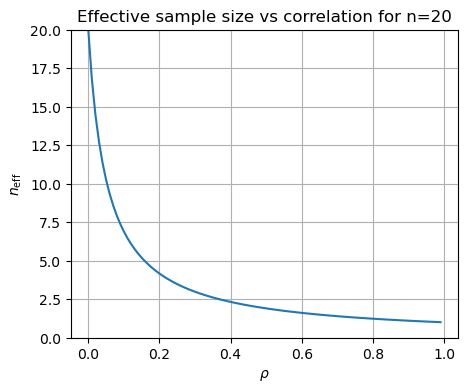
Thus the effective number of degrees of freedom is

\[ n_{\text{eff}} = \frac{n}{[1 + (n-1)\rho]} . \]

This also follows from the Fisher information matrix.

For \(n=20\), \(n_{\text{eff}}\) looks like:

Show code cell source

Hide code cell source

import numpy as np
import matplotlib.pyplot as plt

n = 20
rho_values = np.linspace(0, 0.99, 100)

n_eff = n / (1 + (n-1)*rho_values)

plt.figure(figsize=(5,4))
plt.plot(rho_values, n_eff)
plt.xlabel(r"$\rho$")
plt.ylabel(r"$n_\mathrm{eff}$")
plt.title(f"Effective sample size vs correlation for n={n}")
plt.ylim(0,20)
plt.grid(True)
plt.show()