24.3. Artificial neural networks#
Artificial neural networks are computational systems that can be trained to perform tasks by learning from examples, generally without having to be programmed with any task-specific rules. Its functionality is supposed to mimic a biological neural system, wherein neurons interact by sending signals to each other. In the computer, these signals are generated by mathematical functions in nodes organized in connected layers. All layers can contain an arbitrary number of nodes, and each connection is represented by a weight variable.
](https://ml4a.github.io/images/temp_fig_mnist.png)
Terminology#
When describing a neural network algorithm we typically need to specify three key ingredients:
Architecture
The architecture specifies the topology (the number and connectivity of nodes) and parameters that are involved in the network. For example, the parameters involved in a neural network could be the weights that multiply signals between the neurons, including bias weights, and other parameters determining the form of the activition functions.
Activation rule
Most neural network models have short time-scale dynamics. Local (possibly node-specific) rules define how the activities change in response to signals from other nodes. Typically the activation rules are functions of the weights in the network and possibly other activation-function hyperparameters.
Learning algorithm
The learning algorithm specifies the way in which the neural network’s weights are optimized during training. This learning is usually viewed as taking place on a longer time scale than the one of the activity rule dynamics. Usually the learning rule involve iterative updates that depend on the activities of the neurons. It may also depend on target values supplied by a teacher and on the current values of the weights.
Artificial neurons#
The field of artificial neural networks has a long history of development and is closely connected with the advancement of computer science and computers in general. A model of artificial neurons was first developed by McCulloch and Pitts in 1943 to study signal processing in the brain. Their work has later been refined by others. The general idea is to mimic the functionality of the neural network in the human brain. This biological system is composed of billions of neurons that communicate with each other by sending electrical signals. Each neuron accumulates incoming signals which must exceed an activation threshold to trigger the neuron and yield an output. If the threshold is not overcome, the neuron remains inactive, i.e. has zero output.
This behaviour has inspired a simple mathematical model for an artificial neuron.
where the bias \(b\) is sometimes denoted \(w_0\). Here, the signal \(y\) of an artificial neuron is the output of an activation function, which takes as input a weighted sum of signals \(x_1, \dots ,x_n\) received from \(n\) connected artificial neurons.
Conceptually, it is helpful to divide neural networks into four different categories:
general purpose neural networks, including deep neural networks (DNN) with several hidden layers, for supervised learning,
neural networks designed specifically for image processing, the most prominent example of this class being Convolutional Neural Networks (CNNs),
neural networks for sequential data such as Recurrent Neural Networks (RNNs), and
neural networks for unsupervised learning such as Deep Boltzmann Machines.
Artificial neural networks of all these types have found numerous applications in the natural sciences. For example, they have been applied to detect phase transitions in Ising and Potts models, lattice gauge theories, and classify different phases of polymers. They have been used to simulate solutions to numerous differential equations such as the Navier-Stokes equation in weather forecasting. Deep learning has also found interesting applications in quantum physics. For example, in quantum information theory, it has been shown that one can perform gate decompositions with the help of neural networks.
The scientific applications are certainly not limited to the natural sciences. In fact, there is a plethora of applications in essentially all disciplines, from the humanities to life science and medicine. However, the real expansion has been into the tech industry and other private sectors.
Neural network types#
An artificial neural network is a computational model that consists of layers of connected neurons. We will refer to these computational units as nodes.
A wide variety of different kinds of neural networks have been developed. Most of them are constructed with an input layer, an output layer, and hidden layers in between. All layers contain a number of nodes, and connections between nodes are associated with weight variables.
Neural networks (also called neural nets) can be used as nonlinear models for supervised learning. As we will see, neural networks can be viewed as powerful extensions of supervised learning methods such as linear and logistic regression.
Feed-forward neural networks#
The feed-forward neural network (FFNN) was the first and simplest type of artificial neural network that was devised. In this type of network, the information moves in one direction, namely forward through the layers from input to output.
In Fig. 24.1 the nodes are represented by circles, while the arrows display the connections between the nodes and show the direction of information flow. Additionally, each arrow corresponds to a weight variable. In this network, every node in one layer is connected to all nodes in the subsequent layer, making this a so-called fully-connected FFNN.
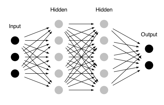
Fig. 24.1 A FFNN with two hidden layers. In addition to the weights associated with the connection arrows there can also be a bias weight connected with each of the active nodes in the hidden and output layers.#
Convolutional Neural Network#
A different variant of FFNNs are convolutional neural networks (CNNs). These networks have a connectivity pattern inspired by the animal visual cortex. Individual neurons in the visual cortex only respond to stimuli from small sub-regions of the visual field, called a receptive field. A similar connectivity of CNNs makes them well-suited to exploit the strong spatial correlations present in images. The response of each node in a CNN is expressed mathematically as a convolution operation.
Convolutional neural networks emulate the behaviour of neurons in the visual cortex by enforcing a local connectivity pattern between nodes of adjacent layers: Each node in a convolutional layer is connected only to a subset of the nodes in the previous layer, in contrast to the fully-connected FFNN. Often, CNNs consist of several convolutional layers that learn local features of the input, with a fully-connected layer at the end, which gathers all the local data and produces the outputs. They have wide applications in image and video recognition.
Recurrent neural networks#
So far we have only mentioned artificial neural networks where information flows only in the forward direction. Recurrent neural networks, on the other hand, have connections between nodes that form directed cycles. This creates a form of internal memory which is able to capture information on what has been calculated before. The output becomes dependent on previous computations. Recurrent neural networks can therefore make use of sequential information. An example of sequential information is sentences, making recurrent neural networks especially well-suited for text and speech recognition.
Feedback networks#
Artificial neural networks that can perform unsupervised learning typically require some sort of feedback mechanism. Two famous examples of feedback networks are Hopfield networks and Boltzmann machines. Due to strong analogies with quantum spin systems, the functionality of these networks can be understood with arguments from statistical physics. This discovery was awarded with the 2025 Nobel Prize in physics.
Neural network architecture#
Let us restrict ourselves in this lecture to fully-connected FFNNs. The term multilayer perceptron is used ambiguously in the literature, sometimes loosely to mean any FFNN, sometimes strictly to refer to networks composed of multiple layers of perceptron nodes (with step-function activation). A general FFNN, however, consists of:
An input layer that distributes the input signals to the active layers.
A multilayer network structure with one or more hidden layers, and one output layer.
the input nodes pass values to the first hidden layer, its nodes pass the information on to the second and so on until the output layer produces the final output.
The number of layers correspond to the network depth. As a convention we primarily count the number of active layers (i.e., those that are associated with activation signals) when specifying the depth. Consequently, we denote a network with one layer of input units plus one layer of hidden units and one layer of output units as a two-layer network. A network with two layers of hidden units is called a three-layer network, etc.
The number of nodes can be different in each layer and is usually known as the layer width. Note, however, the the number of nodes in the input and output layers are dictated by the task, or mapping, that the network should perform. For example, a network that is constructed to describe a relation \(y = y(x_1, x_2)\) will have two input nodes and one output node.
The hidden layers are not linked to observables but play an important role in learning and describing complex relations.
Why deep neural networks?#
According to the universal approximation theorem [Cyb89], a feed-forward neural network with just one hidden layer containing a finite number of neurons can approximate a continuous multidimensional function to arbitrary accuracy. The proof of this theorem assumes that the activation function for the hidden layer is a non-constant, bounded and monotonically-increasing continuous function. The theorem thus states that simple neural networks provide flexible models for a wide variety of interesting functions. The multilayer, feedforward architecture has proven to be easier to train and really gives neural networks the potential of being universal approximators.
Mathematical model#
In a FFNN, the inputs to the nodes in one layer are the outputs of the nodes in the preceding layer.
Starting from the first hidden layer, we compute a weighted sum \(z_j^1\) of the input signals \(\boldsymbol{x} = (x_1, \ldots, x_n)\), for each node \(j\)
where \(w_{ij}^1\) are the linear weights of this node and \(b^1_j\) is known as a bias, or threshold, weight.
The value, \(z_j^1\), is known as the activation and becomes the argument to the activation function \(f^1(z)\) of node \(j\). For simplicity we assume that all nodes in one layer have the same activation function. The output from node \(j\) in the first layer then becomes
When the output of all the nodes in the first hidden layer are computed, the activation of the subsequent layer can be calculated and so forth. Propagating signals from layer to layer we eventually reach node \(j\) in layer \(l\). Its output signal is produced via its activation function \(f^l(z^l_j)\)
where \(N_{l-1}\) is the number of nodes in layer \(l-1\).
The final output (from output node \(i\)) for a neural network with \(L\) hidden layers reads
which illustrates that \(\boldsymbol{y} = (y^{L+1}_1, \ldots, y^{L+1}_m\)) are the dependent variables and the input \(\boldsymbol{x}\) are the independent variables.
This confirms that a FFNN, despite its quite convoluted mathematical form, is nothing more than a non-linear mapping. For example it can map real-valued vectors \(\boldsymbol{x} \in \mathbb{R}^n \rightarrow \boldsymbol{y} \in \mathbb{R}^m\).
Furthermore, the flexibility and universality of a neural network can be illustrated by realizing that the expression is essentially a nested sum of scaled activation functions leading to
where \(\boldsymbol{W}\) contains the weights and biases which are the model parameters.
Matrix-vector notation#
We can introduce a much more convenient matrix-vector notation for all quantities in a FFNN.
In particular, we represent all signals as layer-wise row vectors \(\boldsymbol{y}^l\) so that the \(i\)-th element of each vector is the output \(y_i^l\) of node \(i\) in layer \(l\).
We have that \(\boldsymbol{W}^l\) is an \(N_{l-1} \times N_l\) matrix, while \(\boldsymbol{b}^l\) and \(\boldsymbol{y}^l\) are \(1 \times N_l\) row vectors. With this notation, the sum becomes a matrix-vector multiplication, and we can write the activations of hidden layer \(l\) as
The outputs of this layer then becomes \(\boldsymbol{y}^{l} = f^l(\boldsymbol{z}^{l})\), where we should understand element-wise application of the activation function.
As an example we consider the outputs of the second layer. Assuming three nodes in the first layer we get
This is not just a convenient and compact notation, but also a useful and intuitive way to think about FFNNs. The output is calculated by a sequence of matrix-vector multiplications and vector additions used as input to activation functions.
Activation rules#
A property that characterizes a neural network, other than its connectivity, is the choice of activation function(s). In general, these are non-linear functions. In fact, a FFNN with only linear activation functions would imply that each layer simply performs a linear transformation of its inputs and the output would be an unnecessarily complicated linear mapping of the input.
Logistic and Hyperbolic activation functions. The archetypical example of activation functions is the family of S-shaped (sigmoid) functions. In particular, the logistic (logit) sigmoid function is
and the hyperbolic tangent function is
Noisy networks
Both the sigmoid and tanh activation functions imply that signals will be non-zero everywhere. Even when nodes are inactive, they transmit small, but nonzero, signals. This leads to inefficiencies in both feed-forward and back-propagation operations.
The ambition to completely silence inactive neurons leads to the family of rectifier activation functions. The Rectifier Linear Unit (ReLU) uses the following activation function
However, this type of activation function gives zero gradients, \(f'(z) = 0\) for \(z<0\), which makes weight updates during training much less efficient. To solve this problem, known as dying ReLU neurons, practitioners often use modified versions of the ReLU function, such as the leaky ReLU or the exponential linear unit (ELU) function
The final layer of a neural network has to use an activation function that produces a relevant output signal for the task at hand. For example, the output nodes could employ a linear activation function to give continuous outputs for regression tasks, or a softmax function to provide classification probabilities.
Learning algorithm#
The learning phase (network training) aims to optimize the weights to minimize a problem and data-specific cost function. This task involves multiple choices
Choosing a cost function, \(C(\data, \boldsymbol{W})\) that describe how to compare model outputs with targets from a training data set.
Common cost-function choices include: Mean-squared error (MSE) or Mean-absolute error (MAE) for regression; Cross-entropy or Accuracy for classification.
Weight regularization or random node dropout to avoid overfitting.
The incorporation of physics (model) knowledge in the construction of a more relevant cost function.
Optimization algorithm.
Back-propagation (see below) can be used to compute the gradient of the cost function with respect to the weights. It corresponds to repeated use of the chain rule on the activation functions while traversing the different layers backwards.
The gradient evaluated after each parameter update can be used to iteratively search for a (local) optimum in the high-dimensional space of weights. Popular gradient descent optimizers include:
Standard stochastic gradient descent (SGD), possibly with batches.
Momentum SGD (to incorporate a moving average)
AdaGrad (with per-parameter learning rates)
RMSprop (adapting the learning rates based on RMS gradients)
Adam (a combination of AdaGrad and RMSprop that employs also the second moment of weight gradients).
Splits of data
Training data: used for training.
Validation data: used to monitor learning and to adjust hyperparameters.
Test data: for final test of perfomance.
General remarks on training:
It is critical that neither validation nor test data is used for adjusting the network weights.
Data is often split into batches such that gradients are computed for a batch of data rather than for the full set all at once.
A full pass of all data is known as an epoch. A validation score is often evaluated at the end of each epoch.
Additional “hyperparameters” that can be tuned include:
The number of epochs (overfitting eventually).
The batch size (interplay between stochasticity and efficiency).
Learning rates.
In conclusion, there are many options when designing and training an neural network.
Limitations of supervised learning with deep networks#
Like all statistical methods, supervised learning using neural networks has important limitations. This is especially important when one seeks to apply these methods to physics problems. As all machine-learning algorithms, neural networks are not a universal solution.
As physicists you should always maintain the ambition of learning about the model itself. Often, the same or better performance on a task can be achieved by identifying the most relevant features.
Here we list some of the important limitations of supervised neural network based models.
Need labeled data. All supervised learning methods require labeled data. Often, labeled data is harder to acquire than unlabeled data (e.g. one must pay for human experts to label images).
Deep neural networks are extremely data hungry. They perform best when data is plentiful. This is extra problematic for supervised methods where the data must also be labeled. The utility of deep neural networks is extremely limited if data is hard to acquire or the datasets are small (hundreds to a few thousand samples). In this case, the performance of other methods that utilize hand-engineered features can exceed that of deep neural networks.
Homogeneous data. Almost all deep neural networks deal with homogeneous data of one type. It is very hard to design architectures that mix and match data types (i.e., some continuous and some discrete variables). In some applications, mixed data types is what is required. So called ensemble models, such as random forests or gradient-boosted trees, hare better suited to handle mixed data types.
Many problems are not just about prediction. In the natural sciences we are often interested in learning about the underlying process that generates the data. In this case, it is often difficult to cast hypotheses in a supervised learning setting. While the problems are related, it is possible to make good predictions with a wrong model. The model might or might not be useful for understanding the underlying scientific principles.
Exercises#
Exercise 24.1 (Weights and signal propagation of a simple neural network)
Consider a neural network with two nodes in the input layer, one hidden layer with three nodes, and an output layer with one node (see Fig. 24.2). All active nodes (i.e., those that map input signals to an output via an activation function) employ the same activation function \(f(z) = 1 / (1 + e^{-z})\) and include a bias weight when computing the activation \(z\).
a) How many free (trainable) parameters does this neural network have?
b) Write an explicit expression for the output signal \(y\) from the output node as a function of its weights \((w^2_{11}, w^2_{12},w^2_{13})\), bias weight \(b^2_1\), and the signals \((y^1_1, y^1_2,y^1_3)\) coming from the nodes in the hidden layer.
c) Write a vector expression for the activations \((z^1_1, z^1_2, z^1_3)\) of the three nodes in the hidden layer given a vector of inputs \((x_1, x_2)\) and a matrix that contains the weights of the hidden layer and a vector that contains the bias weights. Be explicit how the weights are ordered in the matrix such that the activation vector can be obtained with matrix-vector operations.
d) How can the above expression be generalized to handle a scenario when there are four instances of input data?
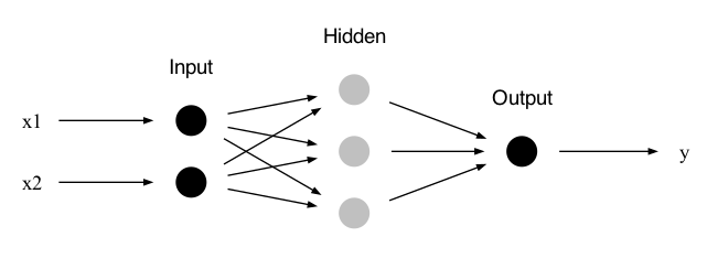
Fig. 24.2 A simple two-layer neural network.#
Exercise 24.2 (Weights and signal propagation of a wide neural network)
Consider a neural network with three nodes in the input layer, one hidden layer with one hundred nodes, and an output layer with two nodes. All nodes in the hidden layer employ the same activation function \(f(z) = 1 / (1 + e^{-z})\) and include a bias weight when computing the activation \(z\). The nodes in the output layer are linear.
a) How many free (trainable) parameters does this neural network have?
b) Introduce relevant matrices and vectors to write down an expression for the output signal \(\boldsymbol{y} = (y_1, y_2)\) given an input \(\boldsymbol{x} = (x_1, x_2, x_3)\).
c) How would this expression have to be modified to handle a scenario when there are \(N\) instances of input data, for which one would like to compute the corresponding network outputs?
Exercise 24.3 (Linear signals)
Consider a neural network with \(p\) nodes in the input layer, one hidden layer with \(L\) nodes, and an output layer with a single node. All nodes in the hidden layer employ the same activation function \(f(z) = 1 / (1 + e^{-z})\) and include a bias weight when computing the activation \(z\). The node in the output layer is linear.
a) Consider small signals and weights such that the output from the nodes in the hidden layer can be approximated by linear functions in the input \(\inputs = (\inputt_1, \inputt_2, \ldots, \inputt_p)\). Write an expression for the output from one of these nodes.
b) Show that the final output from the network also becomes linear in the inputs and relate the coefficients of this expression to the weights of the network.
Exercise 24.4 (Expected signal)
Consider a single node with \(p\) input signals, including a bias weight when computing the activation \(z\), and with a sigmoid activation function \(f(z) = 1 / (1 + e^{-z})\). All weights are initialized as independent draws from a standard normal distribution (zero mean and unit variance).
Assume that you would initialize a large number of instances of this kind of node. Each one will have different weights. For each one, you propagate the same input signal \(\inputs\) and measure the node’s activation \(z\) and output \(y\).
a) How would the distribution \(\p{z}\) of the measured activations look like?
b) How would the distribution \(\p{y}\) of the measured outputs look like?
c) Study the form of \(\p{y}\) for the two different limits \(|\inputs| \ll 1\) (also with \(w_0 \ll 1\)) and \(|\inputs| \gg 1\).
Hints
You can choose to do task c) numerically, which is rather straightforward given that you have solved a) and b), or you can study it analytically which is straightforward for the first case (small signals) but harder for the second one.
For the numerical solution you might have problems with computer precision for large signals. You could consider rewriting your probability distribution, or just consider \(|\inputs| \approx 1\) is large enough to see the appearance of a bimodal distribution.
Solutions#
Solution to Exercise 24.1 (Weights and signal propagation of a simple neural network)
a) Trainable parameters are in the active nodes which, in this case, are the nodes in the hidden layer and the output layer. There are three weights per node in the hidden layer (two linear ones multiplying the two input signals and one bias) and four weights in the output node (three linear weights and one bias). Therefore, in total, there are \(3 \times 3 + 4 = 13\).
b) \(y = 1 / (1+e^{-z})\), where \(z = w^2_{11} y^1_1 + w^2_{12} y^1_2 + w^2_{13} y^1_3 + b^2_1\).
c) \(\boldsymbol{z}^{1} = \boldsymbol{x} \cdot \boldsymbol{W}^{1} + \boldsymbol{b}^{1}\), where \(\boldsymbol{z}^{1} = (z^1_1, z^1_2, z^1_3)\), \(\boldsymbol{x} = (x_1, x_2)\), \(\boldsymbol{b}^{1} = (b^1_1, b^1_2,b^1_3)\) are all row vectors and \(\boldsymbol{W}^{1} = \begin{pmatrix} w^{1}_{11} & w^{1}_{12} & w^{1}_{13} \\ w^{1}_{21} & w^{1}_{22} & w^{1}_{23} \end{pmatrix}\) is a \(2 \times 3\) matrix.
d) It would look the same \(\boldsymbol{Z}^{1} = \boldsymbol{X} \cdot \boldsymbol{W}^{1} + \boldsymbol{b}^{1}\) but \(\boldsymbol{Z}^{1}\) would now be a \(4 \times 3\) matrix with each row containing the hidden layer node activations for the corresponding instance of input data (row in \(\boldsymbol{X}\)). Applying the activation function \(f(z)\) to each element of this matrix would give the corresponding output signals \(\boldsymbol{Y}^{1}\) as another \(4 \times 3\) matrix.
Solution to Exercise 24.2 (Weights and signal propagation of a wide neural network)
a) There are \(100 \times (3+1) + 2 \times (100+1) = 602\) trainable parameters.
b) \(\boldsymbol{y} = \boldsymbol{z} = \boldsymbol{y}^1 \boldsymbol{W}^2 + \boldsymbol{b}^2\), where the output layer parameters appear in the \(\boldsymbol{W}^2\) matrix and the \(\boldsymbol{b}^2\) vector.
Furthermore, \(\boldsymbol{y}^1 = 1 / (1+e^{-\boldsymbol{z}^1})\) and \(\boldsymbol{z}^{1} = \boldsymbol{x} \boldsymbol{W}^{1} + \boldsymbol{b}^{1}\).
The weight matrices and the bias vectors of layer \(L\) have elements \(w^L_{ij}\) and \(b^L_j\), respectively, and will have the sizes: \(\text{dim}(\boldsymbol{W}^{1}) = 3 \times 100\), \(\text{dim}(\boldsymbol{b}^{1}) = 1 \times 100\), \(\text{dim}(\boldsymbol{W}^{2}) = 100 \times 2\), \(\text{dim}(\boldsymbol{b}^{2}) = 1 \times 2\).
c) In this case, the input, \(\boldsymbol{X}\), becomes an \(N \times 3\) matrix. The linear algebra expressions would look the same with the data instances representing one more dimension. That is \(\boldsymbol{Y} = \boldsymbol{Y}^1 \boldsymbol{W}^2 + \boldsymbol{b}^2\), with \(\text{dim}(\boldsymbol{Y}) = N \times 2\), and \(\boldsymbol{Y}^1 = f(\boldsymbol{Z}^1)\). Here, \(\boldsymbol{Z}^{1} = \boldsymbol{X} \boldsymbol{W}^{1} + \boldsymbol{b}^{1}\) is now an \(N \times 3\) matrix with each row containing the hidden layer node activations for the corresponding instance of input data (row in \(\boldsymbol{X}\)). Furthermore, signals \(\boldsymbol{Y}^1\) and activations \(\boldsymbol{Z}^2\) are both matrices with \(N\) rows. Note, however, that the weight and bias matrices are the same.
Solution to Exercise 24.3 (Linear signals)
In the following, superscripts denote the layer with \(l=1\) the hidden layer and \(l=2\) the output layer. Correspondingly, propagating signals are row vectors such that \(w^l_{ij}\) is the weight \(i\) of node \(j\) in layer \(l\) (i.e., it multiplies incoming signal \(i\), \(i=0\) corresponding to the bias).
a) The output of node 1: \(y^1(z^1) = \frac{1}{1+1-z^1+\mathcal{O}((z^1)^2)} = \frac{1}{2} \left( 1 + \frac{z^1}{2} + \mathcal{O}((z^1)^2) \right)\).
With \(z^1 = w^1_{01} + \sum_{i=1}^p w^1_{i1} x_i\) we find
\[ y^1 = \frac{1}{2} + \frac{1}{4} \left( w^1_{01} + \sum_{i=1}^p w^1_{i1} x_i \right). \]b) The final output is \(y = w^2_{01} + \sum_{l=1}^L w^2_{l1} y^1_l\). The signals \(y^1_l\) from the hidden layer are given by (a). We arrive at the linear signal
\[ y = k_0 + k_1 x_1 + k_2 x_2 + \ldots + k_L x_L \]with
\[\begin{split} k_0 &= w^2_{01} + \frac{1}{4} \sum_{l=1}^L w^2_{l1} (2 + w^1_{0l}), \\ k_i &= \frac{1}{4} \sum_{l=1}^L w^2_{l1} w^1_{il}. \end{split}\]
Solution to Exercise 24.4 (Expected signal)
The input is \(\inputs = (\inputt_1, \inputt_2, \ldots, \inputt_p)\) and the node’s weights are \((w_0, w_1, w_2, \ldots, w_p)\) with \(w_0\) the bias.
a) The activation \(z\) will be normally distributed
\[ \p{z} = \mathcal{N}(\mu_z, \sigma_z^2), \]with mean \(\mu_z = 0\) and variance \(\sigma_z^2 = 1 + \left| \inputs \right|^2\).
b) The distribution of the output can be obtained via a transformation \(y = 1 / (1 + e^{-z})\), or rather \(z = \ln (y / (1-y))\). One finds
\[\begin{split} p_Y(y) &= p_Z (z(y)) \left| \frac{d z}{z y} \right| \\ &= \frac{1}{\sqrt{2\pi\sigma_z^2}} \frac{1}{y(1-y)} \exp \left[ -\frac{\left( \ln (y / (1-y)) \right)^2}{2 \sigma_z^2} \right] \end{split}\]c) For small signals the activation will be small and the response will be approximately linear. This means that the final output will be a linear combination of normal-distributed weights, which is another normal distribution. The mode, however, will be at \(y=0.5\).
For very large signals you will find an output distribution that is sharply peaked at \(y=0\) and \(y=1\). That means that you should expect the node to be either very quiet or very noisy, but hardly anything in between (the expectation value will still be \(\expect{y} = 0.5\), but \(\std{y} \to 0.5\).)