8.1. Advantages of the Bayesian approach

“Bayesian inference probabilities are a measure of our state of knowledge about nature, not a measure of nature itself.”

—Devinderjit Sivia

The Bayesian approach offers a number of distinct advantages in scientific applications. Some of them are listed below. In this chapter we introduce in particular the multiple ways of inference with parametric models.

How the Bayesian approach helps in science

1. Provides an elegantly simple and rational approach for answering any scientific question for a given state of information. The procedure is well-defined:

   • Clearly state your question and prior information.

   • Apply the sum and product rules. The starting point is always Bayes’ theorem.

2. Provides a way of eliminating nuisance parameters through marginalization.

   • For some problems, the marginalization can be performed analytically, permitting certain calculations to become computationally tractable.

   • For other problems, sampling is a straightforward way to include many nuisance parameters.

3. Provides a well-defined procedure for propagating errors,

   • E.g., incorporating the effects of systematic errors arising from both the measurement operation and theoretical model predictions.

4. Incorporates relevant prior (e.g., known signal model or known theory model expansion) information through Bayes’ theorem.

   • This is one of the great strengths of Bayesian analysis.

   • Enforces explicit assumptions.

   • For data with a small signal-to-noise ratio, a Bayesian analysis can frequently yield many orders of magnitude improvement in model parameter estimation, through the incorporation of relevant prior information about the signal model.

5. For some problems, a Bayesian analysis may simply lead to a familiar (frequentist) statistic. Even in this situation it often provides a powerful new insight concerning the interpretation of the statistic.

6. Provides a more powerful way of assessing competing theories at the forefront of science by automatically quantifying Occam’s razor.

   • The evidence for two hypotheses or models, \(M_i\) and \(M_j\), can be compared in light of data \(\data\) by evaluating the ratio \(p(M_i|\data, I) / (M_j|\data, I)\).

   • The Bayesian quantitative Occam’s razor can also save a lot of time that might otherwise be spent chasing noise artifacts that masquerade as possible detections of real phenomena.

Occam’s razor

Occam’s razor is a principle attributed to the medieval philosopher William of Occam (or Ockham). The principle states that one should not make more assumptions than the minimum needed. It underlies all scientific modeling and theory building. It cautions us to choose from a set of otherwise equivalent models of a given phenomenon the simplest one. In any given model, Occam’s razor helps us to “shave off” those variables that are not really needed to explain the phenomenon. It was previously thought to be only a qualitative principle.

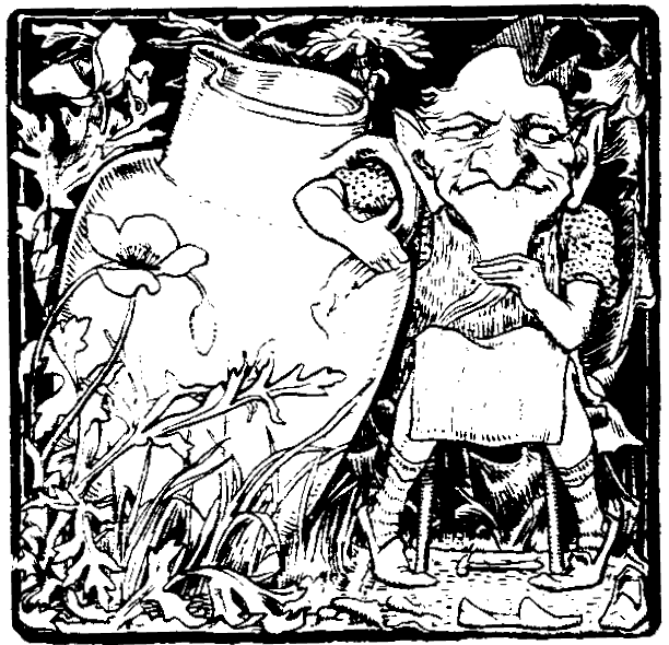
Fig. 8.1 Did the Leprechaun drink your wine, or is there a simpler explanation that does not involve mythical figures?

Inference with parametric models

Inductive inference with parametric models is a very important tool in the natural sciences.

• Consider \(N\) different models \(M_i\) (\(i = 1, \ldots, N\)), each with a parameter vector \(\pars_i\). The number of parameters (length of \(\pars_i\)) might be different for different models. Each of them implies a sampling distribution for possible data

• Consider a scientific model \(M\) with a parameter vector \(\pars\). Together with error models this implies a statistical model that gives a sampling distribution for possible data

(8.1)\[\begin{equation} p(\data|{\pars}, M) \end{equation}\]

• The likelihood function is the pdf of the actual, observed data (\(\data_\mathrm{obs}\)) given a set of parameters \(\boldsymbol{\theta}\):

(8.2)\[\begin{equation} {\mathcal{L}}_i (\pars) \equiv p(\data_\mathrm{obs}|\pars, M) \end{equation}\]

With these ingredients, several types of scientific inquiry can be addressed using a Bayesian framework.

Some key types of Bayesian inference with parametric models

Parameter estimation:

Premise: We have chosen a model (say \(M_1\)) and have access to a set of observed data (\(\data_\mathrm{obs}\))

\(\Rightarrow\) What can we infer about the model parameters \(\boldsymbol{\theta}_1\)?

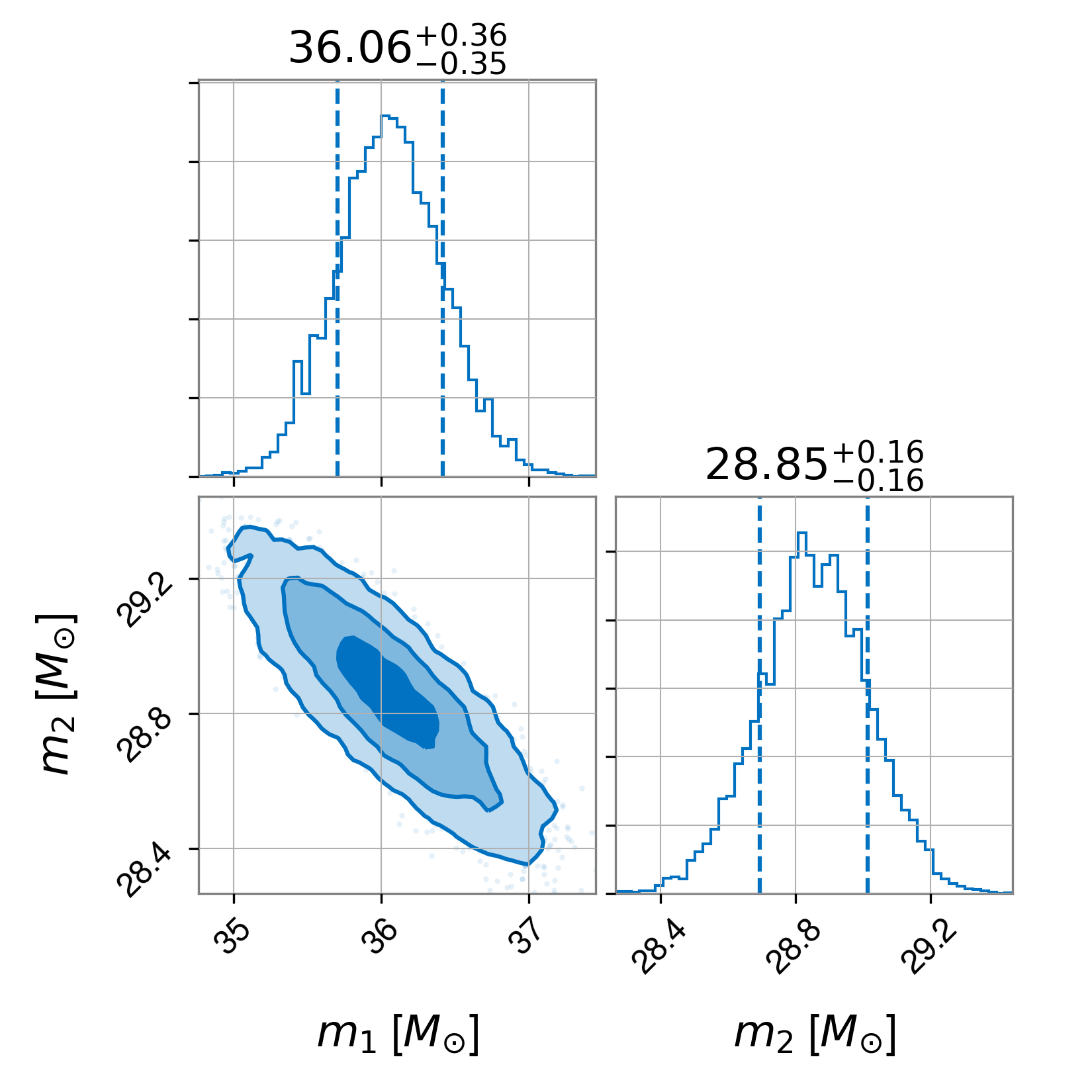
Fig. 8.2 Joint pdf for the masses of two black holes merging obtained from the data analysis of a gravitational wave signal. This representation of a joint pdf is known as a corner plot.

Calibrated model predictions:

Premise: We have a calibrated model (say \(M_1\) and a posterior for parameters \(\boldsymbol{\theta}_1\) given data).

\(\Rightarrow\) What can we predict for new (not measured) data (posterior predictive distribution)?

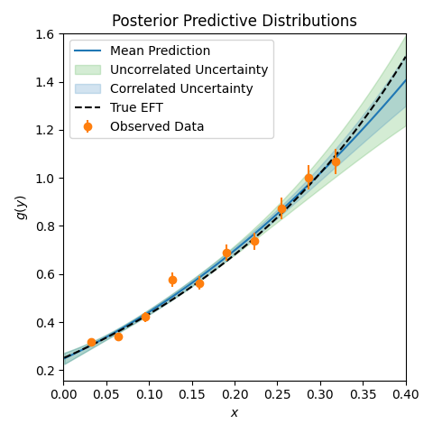
Fig. 8.3 Posterior predictive distributions (ppds) for a toy effective field theory (a truncated Taylor expansion) given data with errors as shown, compared to the true underlying function. The two ppds correspond to including or not including correlations.

Model comparison:

Premise: We have a set of different models, \(\{M_i\}_{i=1}^N\), each with a parameter vector \(\pars_i\). The number of parameters (length of \(\pars_i\)) might be different for different models.

\(\Rightarrow\) How do they compare with each other? Do we have evidence to say that, e.g. \(M_1\), is better than \(M_2\)? Note: better must be defined.

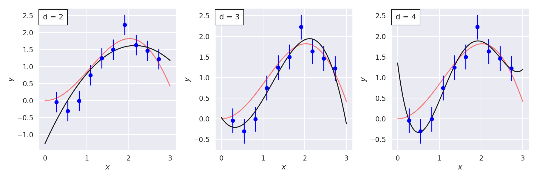
Fig. 8.4 Three polynomial models \(M_1\), \(M_2\), \(M_3\) and their “best fits” to noisy data (the “true” curve is in red). The model comparison problem is to objectively compare the models.

Combining models:

Premise: We have models \(M_1\), \(M_2\), \(M_3\).

\(\Rightarrow\) How can we combine them to make better inferences than any single model?

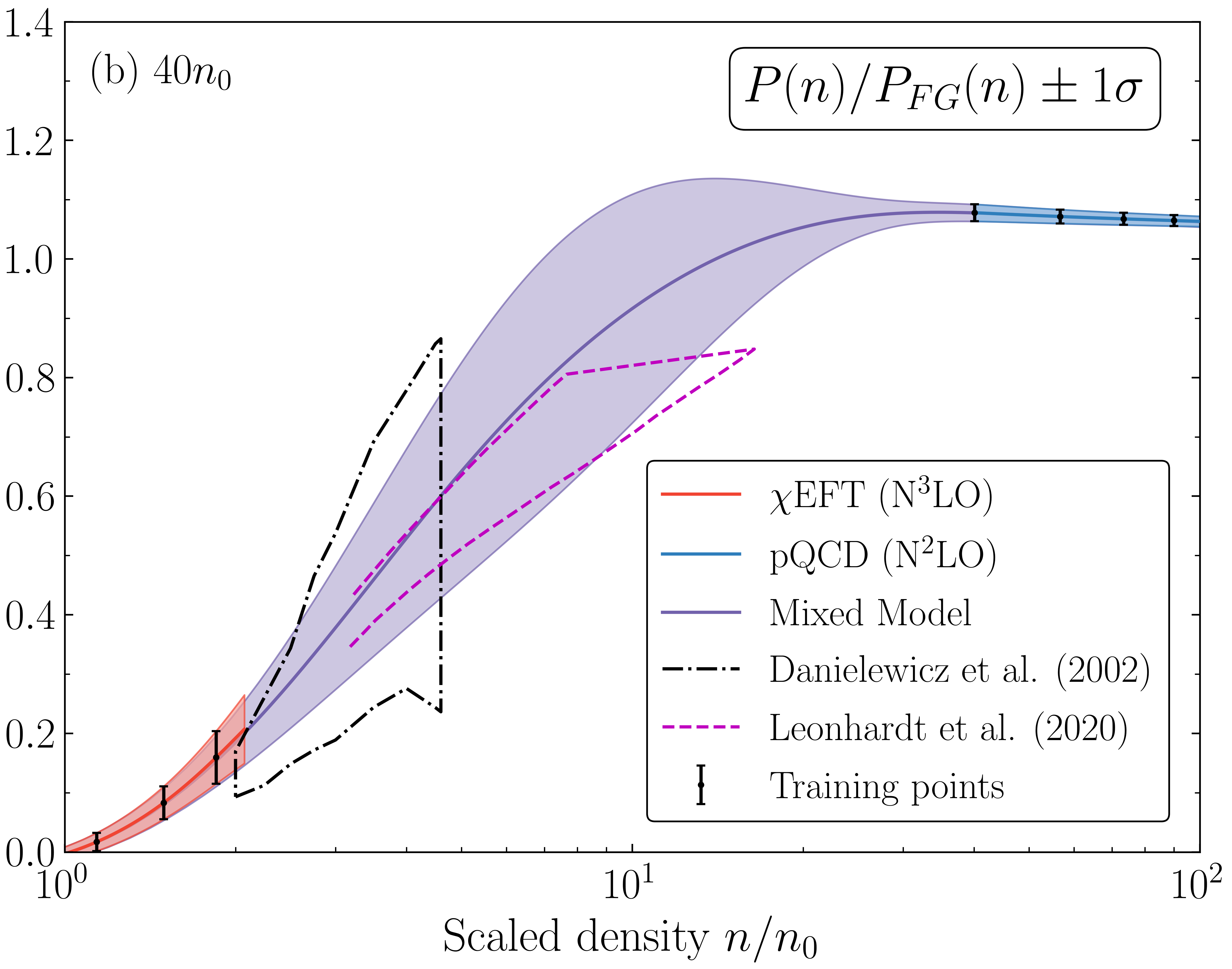
Fig. 8.5 Mixed model equation of state (scaled pressure vs. scaled density) for symmetric nuclear matter. Models with theory errors at low density (red) and very high density (blue) are mixed to bridge the gap between them (purple). One sigma error bands are shown. The figure is from Semposki et al., arxiv:2404.06323.

Experimental design:

Premise: Given a statistical model for experimental predictions.

\(\Rightarrow\) How should we design an experiment to provide the most information for addressing a specific scientific question?

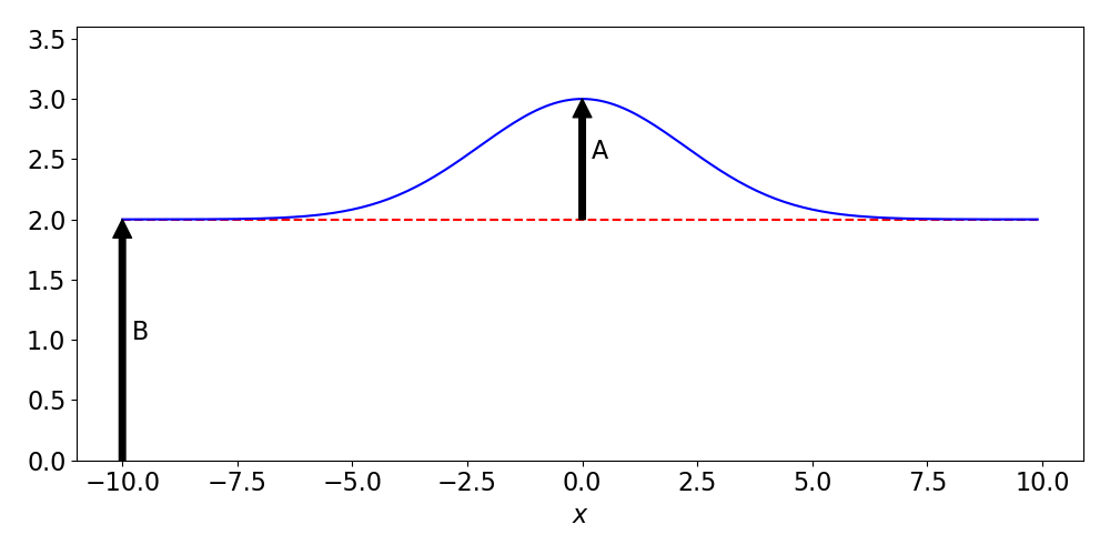
Fig. 8.6 Schematic signal with background from Amplitude of a Signal in the Presence of Background. The experimental design problem is how to best extract the signal properties from optimizing a function that gives the cost of experimental choices, such as the resolution of the detector and the number of counts recorded.

Further discussion on Bayesian approaches to all of these will appear in subsequent chapters.