36. Gradient-descent optimization

With the linear regression model we could find the best fit parameters by solving the normal equation. Although we could encounter problems associated with inverting a matrix, we do in principle have a closed-form expression for the model parameters.

In general, the problem of optimizing the model parameters is a very difficult one. We will return to the optimization problem later in this course, but will just briefly introduce the most common class of optimization algorithms: Gradient descent methods. The general idea of Gradient descent is to tweak parameters iteratively in order to minimize a cost function.

Let us start with a cost function for our model such as the chi-squared function that was introduced in the Linear Regression lecture (but then labeled \(C\)):

(36.1)\[\begin{equation} \chi^2(\boldsymbol{\theta})=\frac{1}{n}\sum_{i=0}^{n-1}\frac{\left(y_i-\tilde{y}_i\right)^2}{\sigma_i^2}=\frac{1}{n}\left\{\left(\boldsymbol{y}-\boldsymbol{\tilde{y}}\right)^T \boldsymbol{\Sigma}^{-1}\left(\boldsymbol{y}-\boldsymbol{\tilde{y}}\right)\right\}, \end{equation}\]

Instead of finding a matrix equation for the vector \(\boldsymbol{\theta}\) that minimizes this measure we will describe an iterative procedure:

• Make a random initialization of the parameter vector \(\boldsymbol{\theta}_0\).

• Compute the gradient of the cost function with respect to the parameters (note that this can be done analytically for the linear regression model). Let us denote this gradient vector \(\boldsymbol{\nabla}_{\boldsymbol{\theta}} \left( \chi^2 \right)\).

• Once you have the gradient vector, which points uphill, just go in the opposite direction to go downhill. This means subtracting \(\eta \boldsymbol{\nabla}_{\boldsymbol{\theta}} \left( \chi^2 \right)\) from \(\boldsymbol{\theta}_0\). Note that the magnitude of the step, \(\eta\) is known as the learning rate and becomes another hyperparameter that needs to be tuned.

• Continue this process iteratively until the gradient vector \(\boldsymbol{\nabla}_{\boldsymbol{\theta}} \left( \chi^2 \right)\) is close to zero.

Gradient descent is a general optimization algorithm. However, there are several important issues that should be known before using it:

1. It requires the computation of partial derivatives of the cost function. This is straight-forward for the linear regression method, see Eq. (39.17), but can be difficult for other models. The use of automatic differentiation is very popular in the ML community,and is well worth exploring.

2. In principle, gradient descent works well for convex cost functions, i.e. where the gradient will eventually direct you to the position of the global minimum. Again, the linear regression problem is favorable because you can show that the cost function has that property. However, most cost functions—in particular in many dimensions—correspond to very complicated surfaces with many local minima. In those cases, gradient descent is often not a good method.

There are variations of gradient descent that uses only fractions of the training set for computation of the gradient. In particular, stochastic gradient descent and mini-batch gradient descent.

36.1. Learning curves

The performance of your model will depend on the amount of data that is used for training. When using iterative optimization approaches, such as gradient descent, it will also depend on the number of training iterations. In order to monitor this dependence one usually plots learning curves.

Learning curves are plots of the model’s performance on both the training and the validation sets, measured by some performance metric such as the mean squared error. This measure is plotted as a function of the size of the training set, or alternatively as a function of the training iterations.

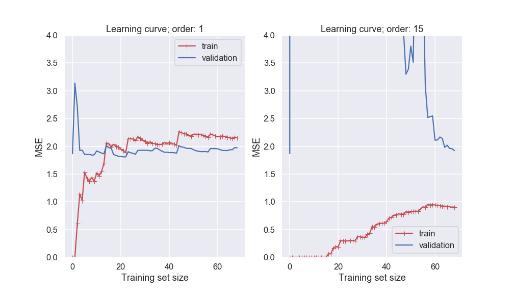
Fig. 36.1 Learning curves for different polynomial models of our noisy data set as a function of the size of the training data set.

Several features in the left-hand panel deserves to be mentioned:

1. The performance on the training set starts at zero when only 1-2 data are in the training set.

2. The error on the training set then increases steadily as more data is added.

3. It finally reaches a plateau.

4. The validation error is initially very high, but reaches a plateau that is very close to the training error.

The learning curves in the right hand panel are similar to the underfitting model; but there are some important differences:

1. The training error is much smaller than with the linear model.

2. There is no clear plateau.

3. There is a gap between the curves, which implies that the model performs significantly better on the training data than on the validation set.

Both these examples that we have just studied demonstrate again the so called bias-variance tradeoff.

• A high bias model has a relatively large error, most probably due to wrong assumptions about the data features.

• A high variance model is excessively sensitive to small variations in the training data.

• The irreducible error is due to the noisiness of the data itself. It can only be reduced by obtaining better data.

We seek a more systematic way of distinguishing between under- and overfitting models, and for quantification of the different kinds of errors. We will find that Bayesian statistics has the promise to deliver on that ultimate goal.