17.2. Basic structure and intuition for MH#
Basic structure of Metropolis-Hastings algorithm#
Let’s elaborate on the structure of the MCMC algorithm.
Given \(\thetavec_i\), propose a value for \(\thetavec_{i+1}\), call it the “candidate” \(\phivec\), sampled from \(q(\phivec|\thetavec_i)\). This \(q\) could take many forms, so for concreteness imagine it as a multivariate normal distribution with mean given by \(\thetavec_i\) and variance \(\sigmavec^2\) (to be specified). This entails a decreased probability to step further away from the current sample and \(\sigmavec\) sets scale of the step size.
Decide whether or not to accept candidate \(\phivec\) for \(\thetavec_{i+1}\). Here we’ll use the Metropolis condition (later we’ll see other ways that may be better). This approach dates from the 1950’s in physics but didn’t become widespread in statistics until almost 1980. With its adoption, it finally enabled Bayesian methods to be much more widely applied.
Metropolis condition
Calculate Metropolis ratio \(r\) given current \(\thetavec_i\) and proposed candidate \(\phivec\):
The distribution \(q\) may be symmetric: \(q(\thetavec_1|\thetavec_2) = q(\thetavec_2|\thetavec_1)\). If so, then this is called “Metropolis”. If not, then it is called “Metropolis-Hastings”.
Decision:
If \(r\geq 1\), set \(\thetavec_{i+1} = \phivec\) \(\Lra\) always accept
If \(r < 1\), so less probable, don’t always reject! Accept with probability \(r\) by sampling a Uniform (0,1) distribution. (Because \(0\leq r\leq 1\) for this case we can take \(r\) as a probability.)
In practice we carry out the \(r<1\) case by getting a sample \(U \sim \text{Uniform}(0,1)\). If \(U \leq r\), then \(\thetavec_{i+1} = \phivec\), else \(\thetavec_{i+1} = \thetavec_i\).
Note that the last case means you do have a \(\theta_{i+1}\), but it is the same as \(\theta_i\), so you have multiple copies and the chain always continues to grow. We further note that the acceptance probability is the minimum of \(1\) and \(r\), which makes the (pseudo-)code particularly simple:
Algorithm pseudo-code:
Initialize \(\thetavec_i\), set \(i=0\).
Repeat
{
Obtain new candidate \(\phivec\) from \(q(\phivec|\theta_i)\) Calculate \(r\) Sample \(U \sim \text{uniform}(0,1)\) If \(U \leq r\) set \(\thetavec_{i+1} = \phivec\), else set \(\thetavec_{i+1} = \thetavec_i\).
\(i++\)
}
It’s important to do the else step for \(U \gt r\) (see below).
Intuition for detailed balance and the MH algorithm#
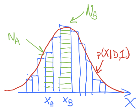
Imagine the schematic histogram here is the accumulated distribution of walkers after some time. The red line is the posterior we are sampling, \(p(X|D,I)\) (we’re using \(X\) instead of \(\thetavec\) for a change of pace), so it is looking like we have an equilibrated distribution (more or less). This doesn’t mean the distribution is static as we continue to sample; walkers will continue to roam around and we’ll accumulate more green boxes at different \(X\) values. But if our Metropolis-Hastings algorithm is correctly implemented, the histogram shape should be stationary at the correct posterior, i.e., it should not change with time except for fluctuations.
After equilibrium we look at the chain and note there are \(N_A\) green boxes at \(X_A\) and \(N_B\) green boxes at \(X_B\). Let’s consider each of the \(X_A\) boxes in turn in the chain. Each of the boxes at \(X_A\) had a chance with the next Monte Carlo step to go to \(X_B\). Similarly, each of the boxes at \(X_B\) had a chance to go to \(X_A\). For a steady-state situation, we need the number of actual moves in each direction to be the same. This means that the two rates of all such transitions are equal; this is what we mean by “detailed balance”.
Checkpoint question
What if the only moves accepted were those that went uphill (i.e., to higher probability density)? What would happen to \(N_A\) and \(N_B\) over time? Is this stationary?
Answer
If only uphill move were accepted, then \(N_B\) would monotonically increase while \(N_A\) would eventually monotonically decrease (it would get some input at first from lower probability values of \(X\) but eventually those would all be gone). So all of the boxes would end up at \(x_B\). This is stationary but not at the posterior we are sampling!
Ok, so suppose \(p(X|X')\) is the transition probability, that we’ll move from \(X'\) to \(X\).
Checkpoint question
In terms of \(p(X_A|X_B)\), \(p(X_B|X_A)\), \(N_A\), and \(N_B\), what is the condition that the exchanges between \(A\) and \(B\) cancel out? (For now assume a symmetric proposal distribution \(q\).)
Answer
Checkpoint question
How are \(N_A\) and \(N_B\) related to the total \(N\) and the posteriors \(p(X_A|D,I)\) and \(p(X_B|D,I)\)?
Answer
Now let’s put it together.
Checkpoint question
What is the ratio of \(p(X_B|X_A)\) to \(p(X_A|X_B)\) in terms of \(p(X_A|D,I)\) and \(p(X_B|D,I)\)?
Answer
Now how do we realize a rule that satisfies the condition we just derived? We actually have a lot of freedom in doing so and the Metropolis choice is just one possibility. Let’s verify that it works. The Metropolis algorithm says
Let’s check cases and see if it works. Here is a chart:
\(p(X_B\vert X_A)\) |
\(p(X_A\vert X_B)\) |
|
|---|---|---|
\(p(X_B\vert D,I) \lt p(X_A\vert D,I)\) |
[fill in here] |
[fill in here] |
\(p(X_A\vert D,I) \lt p(X_B\vert D,I)\) |
[fill in here] |
[fill in here] |
Checkpoint question
Fill in the chart based on the Metropolis algorithm we are using and verify that the ratio of \(p(X_B|X_A)\) to \(p(X_A|X_B)\) agrees with the answer derived above.
Answer
\(p(X_B\vert X_A)\) |
\(p(X_A\vert X_B)\) |
|
|---|---|---|
\(p(X_B\vert D,I) \lt p(X_A\vert D,I)\) |
\(\frac{\displaystyle p(X_B\vert D,I)}{\displaystyle p(X_A\vert D,I)}\) |
1 |
\(p(X_A\vert D,I) \lt p(X_B\vert D,I)\) |
1 |
\(\frac{\displaystyle p(X_A\vert D,I)}{\displaystyle p(X_B\vert D,I)}\) |
Dividing the 2nd by the 3rd columns for the 2nd and 3rd rows each gives the correct result!
Ok, so it works. What if we have an asymmetric proposal distribution? So \(q(X|X') \neq q(X'|X)\). Then we just need to go back to where we were equating rates and add the \(q\)s to each side of the equation. The bottom line is the Metropolis algorithm with the Metropolis ratio \(r\) as we have summarized it at the beginning of this lecture.
Checkpoint question
Why do you think that this property is called detailed balance? Can you make an analogy with thermodynamic equilibrium for a collection of hydrogen atoms?
Answer
At an equilibrium temperature \(T\), the different atoms will be distributed in different energy states according to the Boltzmann distribution. But equilibrium does not mean static; there are constant excitation and de-excitation transitions among the hydrogen atoms. Detailed balance requires that the forward and reverse rates of each particular microscopic transition are equal.
Summary: Metropolis algorithm for \(p(\thetavec | D, I)\) (or any other posterior).
start with inital point \(\thetavec_0\) (for each walker)
begin repeat: given \(\thetavec_i\), propose \(\phivec\) from \(q(\phivec|\thetavec_i)\)
calculate \(r\):
where the left factor compares posteriors and the right factor is a correction for \(r\) if the \(q\) pdf is not symmetric: \(q(\phivec|\thetavec_i) \neq q(\thetavec_i|\phivec)\)
decide whether to keep \(\phivec\):
if \(r\geq 1\), set \(\thetavec_{i+1} = \phivec\) (accept)
else draw \(u \sim \text{uniform}(0,1)\)
if \(u \leq r\), \(\thetavec_{i+1} = \phivec\) (accept)
else \(\thetavec_{i+1} = \thetavec_i\) (add another copy of \(\thetavec_i\) to the chain)
end repeat when “converged”.
Key questions: When are you converged? How many “warm-up” or “burn-in “ steps to skip?
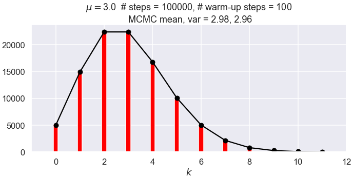
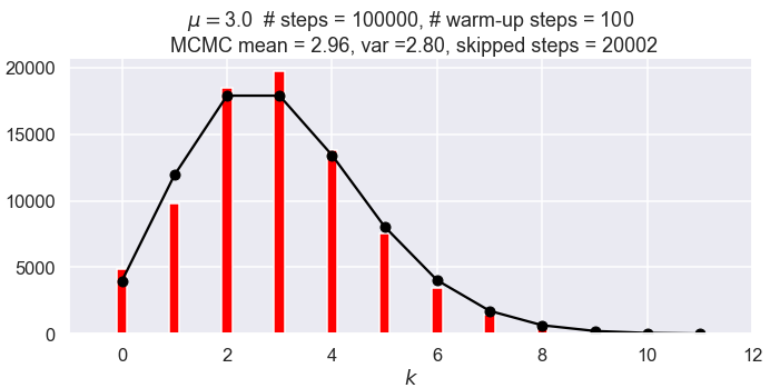
Repeating configurations#
What if the \(\thetavec_{i+1}=\thetavec_i\) step is not implemented as it should be? I.e., what if the chain is only incremented if the step is accepted? You might find that this is more intuitive to you. But consider an empirical demonstration: see the figures below from the Poisson distribution example with 100,000 steps. The first one follows the Metropolis algorithm and adds the same step if the candidate is rejected; the second one does not. Not keeping the repeated steps invalidates the Markov chain conditions \(\Lra\) the wrong stationary distribution is reached (it is not wrong by a lot but is is noticeable and is seen every time the sampling is run).