25.5. MNIST classifier in PyTorch#
This notebook is a PyTorch rewrite of the original TensorFlow/Keras demo.
It trains a simple fully-connected network on MNIST and reproduces:
data loading
model definition (Flatten → Dense(128, ReLU) → Dropout(0.2) → Dense(10))
training for 10 epochs
accuracy on the test set
probability predictions for a sample
the same plotting helpers for predictions
# Imports
import os, math, numpy as np


import torch
from torch import nn
from torch.utils.data import DataLoader
from torchvision import datasets, transforms
import matplotlib.pyplot as plt

print('You have PyTorch version:', torch.__version__)
device = torch.device('cuda' if torch.cuda.is_available() else 'cpu')
print('Using device:', device)
torch.manual_seed(1234)
You have PyTorch version: 2.9.1
Using device: cpu
<torch._C.Generator at 0x7fc3a0b17070>
# Data: MNIST via torchvision (returns tensors in [0,1])
batch_size = 128

transform = transforms.ToTensor()  # simple scaling to [0,1]
train_dataset = datasets.MNIST(root='./data', train=True, download=True, transform=transform)
test_dataset  = datasets.MNIST(root='./data', train=False, download=True, transform=transform)

x_train = train_dataset.data.numpy()
y_train = train_dataset.targets.numpy()
x_test  = test_dataset.data.numpy()
y_test  = test_dataset.targets.numpy()

train_loader = DataLoader(train_dataset, batch_size=batch_size, shuffle=True, num_workers=2)
test_loader  = DataLoader(test_dataset, batch_size=batch_size, shuffle=False, num_workers=2)

print('Train:', len(train_dataset), 'Test:', len(test_dataset))
Train: 60000 Test: 10000
# Model: Flatten → Linear(784,128) → ReLU → Dropout(0.2) → Linear(128,10)
class MLP(nn.Module):
    def __init__(self):
        super().__init__()
        self.net = nn.Sequential(
            nn.Flatten(),
            nn.Linear(28*28, 128),
            nn.ReLU(),
            nn.Dropout(0.2),
            nn.Linear(128, 10)
        )
    def forward(self, x):
        return self.net(x)

model = MLP().to(device)
sum(p.numel() for p in model.parameters()), model
(101770,
 MLP(
   (net): Sequential(
     (0): Flatten(start_dim=1, end_dim=-1)
     (1): Linear(in_features=784, out_features=128, bias=True)
     (2): ReLU()
     (3): Dropout(p=0.2, inplace=False)
     (4): Linear(in_features=128, out_features=10, bias=True)
   )
 ))
# Training
criterion = nn.CrossEntropyLoss()  # expects raw logits
optimizer = torch.optim.Adam(model.parameters())
epochs = 10

history = {'accuracy': [], 'loss': []}

for epoch in range(1, epochs+1):
    model.train()
    running_loss = 0.0
    correct, total = 0, 0
    for xb, yb in train_loader:
        xb, yb = xb.to(device), yb.to(device)
        optimizer.zero_grad()
        logits = model(xb)
        loss = criterion(logits, yb)
        loss.backward()
        optimizer.step()
        running_loss += loss.item() * xb.size(0)

        # compute training accuracy
        preds = logits.argmax(dim=1)
        correct += (preds == yb).sum().item()
        total += yb.size(0)

    epoch_loss = running_loss / total
    epoch_acc = correct / total
    history['loss'].append(epoch_loss)
    history['accuracy'].append(epoch_acc)
    print(f'Epoch {epoch:2d}/{epochs} - loss: {epoch_loss:.4f} - acc: {epoch_acc:.4f}')

history
Epoch 1/10 - loss: 0.4464 - acc: 0.8796
Epoch 2/10 - loss: 0.2149 - acc: 0.9373
Epoch 3/10 - loss: 0.1596 - acc: 0.9535
Epoch 4/10 - loss: 0.1290 - acc: 0.9617
Epoch 5/10 - loss: 0.1077 - acc: 0.9687
Epoch 6/10 - loss: 0.0928 - acc: 0.9725
Epoch 7/10 - loss: 0.0822 - acc: 0.9751
Epoch 8/10 - loss: 0.0748 - acc: 0.9772
Epoch 9/10 - loss: 0.0672 - acc: 0.9794
Epoch 10/10 - loss: 0.0591 - acc: 0.9823
{'accuracy': [0.8795666666666667,
  0.9372833333333334,
  0.95345,
  0.9617,
  0.9687166666666667,
  0.9725,
  0.97515,
  0.9772333333333333,
  0.9794,
  0.9823],
 'loss': [0.4463983178456624,
  0.21493444612026213,
  0.1596157058954239,
  0.1290262913386027,
  0.10767514850695928,
  0.09282231144507726,
  0.08220300891399383,
  0.07477020881772041,
  0.06717816098332405,
  0.05907997849583626]}
# Evaluation on test set
model.eval()
correct, total, test_loss = 0, 0, 0.0
with torch.no_grad():
    for xb, yb in test_loader:
        xb, yb = xb.to(device), yb.to(device)
        logits = model(xb)
        loss = criterion(logits, yb)
        test_loss += loss.item() * xb.size(0)
        preds = logits.argmax(dim=1)
        correct += (preds == yb).sum().item()
        total += yb.size(0)

test_acc = correct / total
test_loss = test_loss / total
print(f'\nTest accuracy: {test_acc:5.3f}')
test_acc
Test accuracy: 0.978
0.9775
# Predict class probabilities for the first test image (to mirror Keras softmax output)
softmax = nn.Softmax(dim=1)
model.eval()
with torch.no_grad():
    sample = test_dataset[0][0].unsqueeze(0).to(device)  # 1x1x28x28
    probs = softmax(model(sample)).cpu().numpy()[0]

probs, probs.sum(), probs.argmax()
(array([3.6496281e-06, 6.8333939e-08, 1.1807497e-05, 5.3805462e-04,
        5.3760618e-10, 1.7252582e-06, 1.9389098e-13, 9.9938619e-01,
        2.5817704e-07, 5.8283444e-05], dtype=float32),
 1.0,
 7)
# Helper plotting functions (ported from the Keras version)
def plot_image(i, predictions_array, true_label, img):
    predictions_array, true_label, img = predictions_array, int(true_label), img
    plt.grid(False)
    plt.xticks([])
    plt.yticks([])

    plt.imshow(img, cmap=plt.cm.binary)
    predicted_label = int(np.argmax(predictions_array))
    color = 'blue' if predicted_label == true_label else 'red'
    plt.xlabel(f"{predicted_label} {100*np.max(predictions_array):2.0f}% (true: {true_label})", color=color)

def plot_value_array(i, predictions_array, true_label):
    predictions_array, true_label = predictions_array, int(true_label)
    plt.grid(False)
    plt.xticks(range(10))
    plt.yticks([])
    thisplot = plt.bar(range(10), predictions_array)
    predicted_label = int(np.argmax(predictions_array))
    thisplot[predicted_label].set_color('red')
    thisplot[true_label].set_color('green')
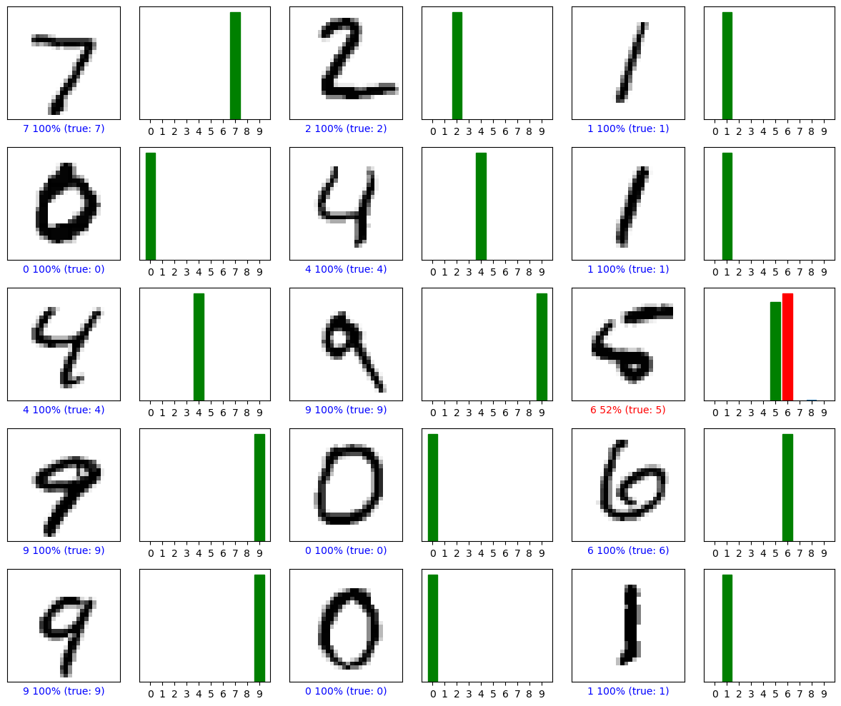
# Plot a grid of test images with predicted probabilities
num_rows = 5
num_cols = 3
num_images = num_rows * num_cols
plt.figure(figsize=(2*2*num_cols, 2*num_rows))

# Precompute probabilities for first num_images
with torch.no_grad():
    xs = torch.stack([test_dataset[i][0] for i in range(num_images)]).to(device)
    probs_batch = nn.Softmax(dim=1)(model(xs)).cpu().numpy()

for i in range(num_images):
    img, label = test_dataset[i]
    plt.subplot(num_rows, 2*num_cols, 2*i+1)
    plot_image(i, probs_batch[i], label, img.squeeze().numpy())
    plt.subplot(num_rows, 2*num_cols, 2*i+2)
    plot_value_array(i, probs_batch[i], label)

plt.tight_layout()
plt.show()