11.4. Real-world application of discrepancy model

These figures are from two papers by Sunil Jaiswal and collaborators, which apply discrepancy models based on Gaussian processes to data from relativistic heavy-ion collisions. The goal is to extract meaningful distributions for the bulk and shear specific viscosities (“specific” in this context means normalized by the entropy density).

Bayesian model-data comparison incorporating theoretical uncertainties

Sunil Jaiswala, Chun Shen, Richard J. Furnstahl, Ulrich Heinz, Matthew T. Pratola, arXiv:2504.13144.

In the following examples we simulate collisions of Au on Au nuclei at \(\sqrt{s_\textrm{NN}} =200\,\)GeV at \(20-30\%\) collision centrality, using the iEBE-MUSIC simulation framework. These simulations are considered to represent the “truth”. We use them to generate mock experimental data. The theoretical model to be compared with these mock data is the same iEBE-MUSIC model but with a different ansatz for the momentum distribution at particlization (assuming local thermal equilibrium \(f_{\text{eq}}\) instead of the Grad 14-moment momentum distributions for the particlized hadrons).

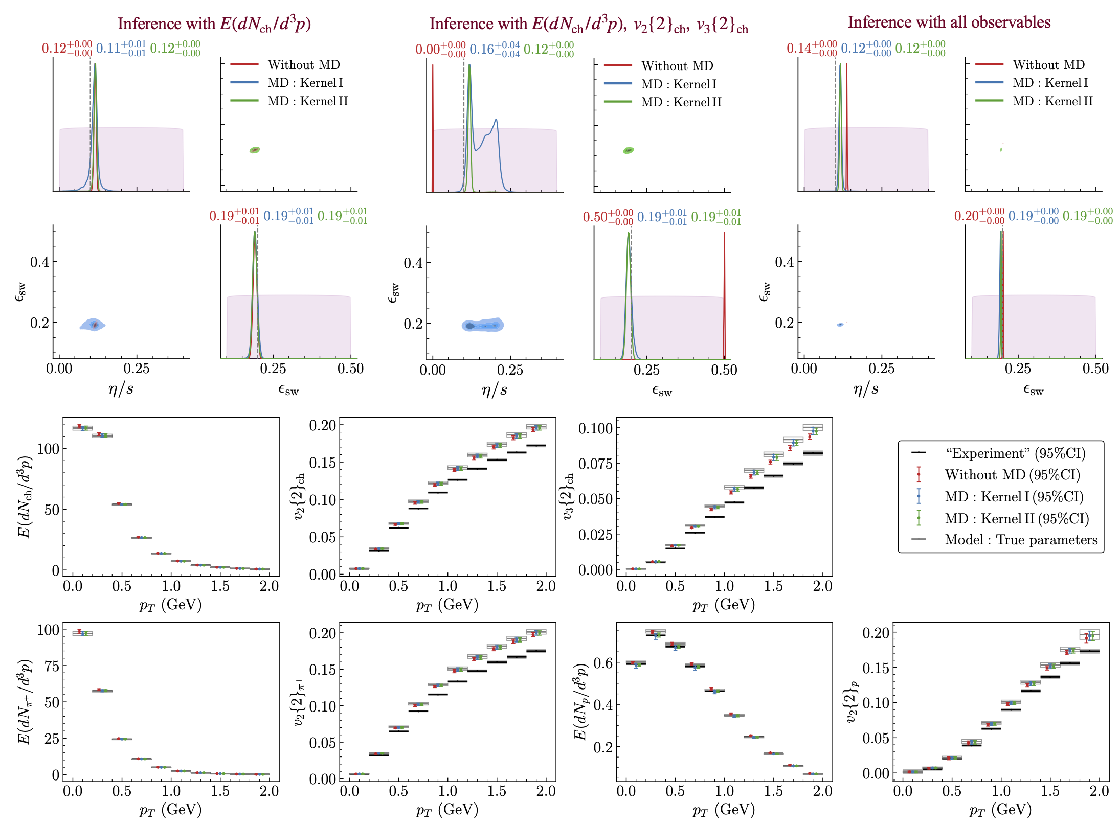
Fig. 11.8 Results for the two-parameter hydrodynamic simulation using mock data generated with fixed \(\eta/s = 0.1\) and \(\epsilon_{\text{sw}} = 0.2 \text{GeV/fm}^3\). Top row: Corner plots showing the posteriors for the inferred \(\eta/s\) and \(\epsilon_{\text{sw}}\) (with median \(\pm 68\%\) CI displayed on the diagonals) as more observables are included in the Bayesian inference (from left to right). Bottom rows: Model predictions based on inference using all observables.

Using only the \(E(dN_{\text{ch}}/d^3p)\) measurements (top left), all three cases (i)-(iii) yield posteriors that are statistically consistent with the truth. However, once the flow observables \(v_2\{2\}_{\rm ch}\) and \(v_3\{2\}_{\rm ch}\) are included (top middle), in the no-MD case (red) the Bayesian fit clearly struggles to find optimal values for the parameters, producing significantly shifted posteriors that hit the edge of the prior range (“very wrong”) while exhibiting exceedingly small uncertainties (“very confident”). Including MD using Kernel I (blue), the posteriors are once again statistically consistent with the truth, albeit with increased uncertainty (“much less confidence”) for \(\eta/s\). With Kernel II (green) the MD term captures the model imperfections for \(v_2\) and \(v_3\) much better, yielding posteriors similar to those obtained by ignoring the charged hadron anisotropic flow data. Once all available observables are included (top right), the inferred values for both model parameters agree with their true values, within significantly reduced uncertainties, as long as MD is accounted for (blue and green); without MD \(\eta/s\) is very confidently inferred to be about \(40\%\) larger than its true value.

The bottom panel of Fig. 11.8 compares the mock experimental data with their predictions from the calibrated model. Black boxes denote the median and \(95\%\) credible intervals (CI) of the experimental data, while open gray boxes show predictions from the model using the true parameter values, the difference highlighting the effects of model imperfections. The colored (red, blue, green) points and vertical bars show the median and \(95\%\) CI of the model predictions obtained from the inferred posteriors in the top right panel. Overall, predictions with MD (blue and green) are closer to the model predictions with the true parameters while those without MD (red) align more closely with the data. This demonstrates that the MD framework prioritizes obtaining correct parameter estimates over merely fitting the observables.

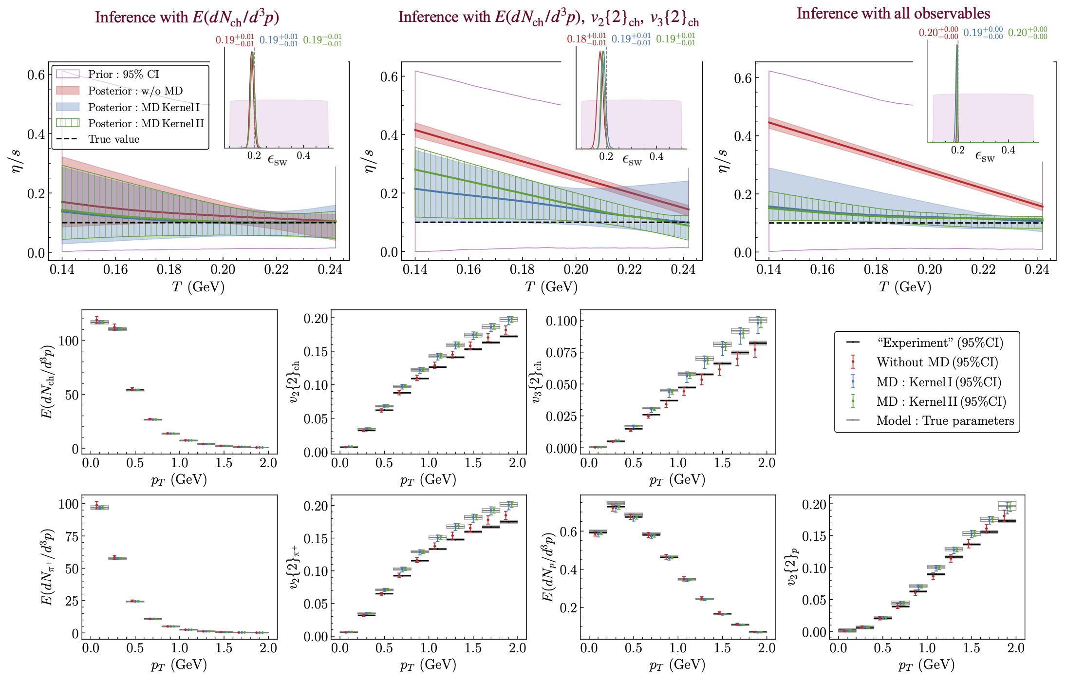
Fig. 11.9 Results for the five-parameter hydrodynamic simulation with parametrized \(\eta/s\) using mock data generated with fixed \(\eta/s=0.1\) and \(\epsilon_{\rm sw}=0.2\,\)GeV/fm\(^3\). Top row: Plots display the \(\eta/s\) posterior (median and \(\pm 95\%\) CI) as a function of temperature, with the posterior for \(\epsilon_{\rm sw}\) (median \(\pm 68\%\) CI) shown in the inset, as additional observables are sequentially incorporated into the Bayesian inference (from left to right). Bottom rows: Model predictions based on inference using all observables.

When only the momentum distribution \(E(dN_{\text{ch}}/d^3p)\) is considered (top left), all three cases yield posteriors that are statistically compatible with the truth. However, for \(\eta/s\) the posteriors accounting for MD (blue and green) overlap significantly better with the true values than those without MD (red). Once \(v_2\{2\}_{\rm ch}\) and \(v_3\{2\}_{\rm ch}\) are added to the calibration data (top middle), none of the posteriors uniformly covers the truth any more. When not accounting for MD (red), the posterior credible intervals for \(\eta/s\) are very narrow (suggesting high confidence) but are completely inconsistent with the truth. Including MD helps a little but still infers \(95\%\) credible intervals that do not cover the true value of \(\eta/s\) over most of the temperature range. Apparently, the inference algorithm tries to compensate for the model’s tendency to over-predict \(v_2\) and \(v_3\) by increasing \(\eta/s\). When all observables (including the spectra and elliptic flows of identified pions and protons) are added to the calibration data (top right), all posteriors become narrower (i.e., more constrained). The overlap of the posteriors accounting for MD improves, whereas the posteriors that do not account for MD degrade further.

The model predictions in the bottom row of Fig. 11.11 (obtained from the inferred posteriors in the top right panel) reinforce our observations made in the two-parameter case: Predictions that include MD do not attempt to overfit the data (black) but remain closer to the model predictions using the true parameter values (open gray). In contrast, the predictions without MD overfit the data, resulting in the incorrect inference for \(\eta/s\) observed in the top right panel.

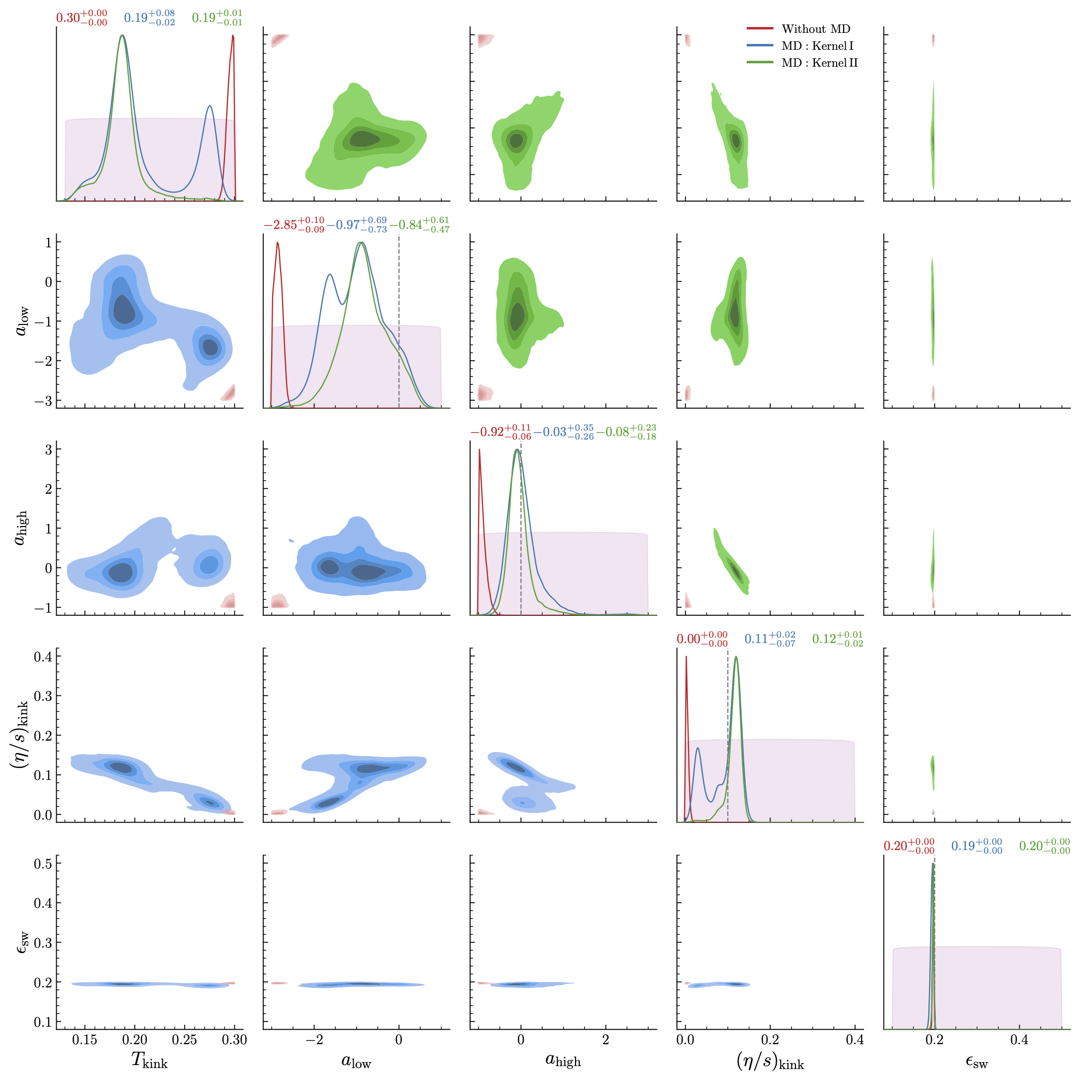
Fig. 11.10 Corner plot of all model parameters (with median \(\pm 68\%\) CI displayed on the diagonals) for the five-parameter model with parametrized \(\eta/s\), using mock data generated with fixed \(\eta/s=0.1\) and \(\epsilon_{\rm sw}=0.2\,\)GeV/fm\(^3\), corresponding to the results shown in Fig. 11.9

Overall, the posteriors agree better with the true values (indicated by dashed gray vertical lines) when the model discrepancy (MD) term is included (for both Kernel I and Kernel II) compared to the no-MD case (red). Note that, since the generated mock experimental data do not depend on the parameter \(T_{\rm kink}\), its posterior should ideally mirror the prior (shaded purple region). However, we observe that the posterior for \(T_{\rm kink}\) peaks around a certain value even in the MD inference, although its width is significantly larger than in the no-MD case. This may be an artifact of the overly flexible model, where the MD cases struggle to disentangle the effects of the model parameter from the GP hyperparameters. Nonetheless, the resulting \(\eta/s\) posterior shown in Fig. 11.9 does not appear to depend crucially on this parameter.

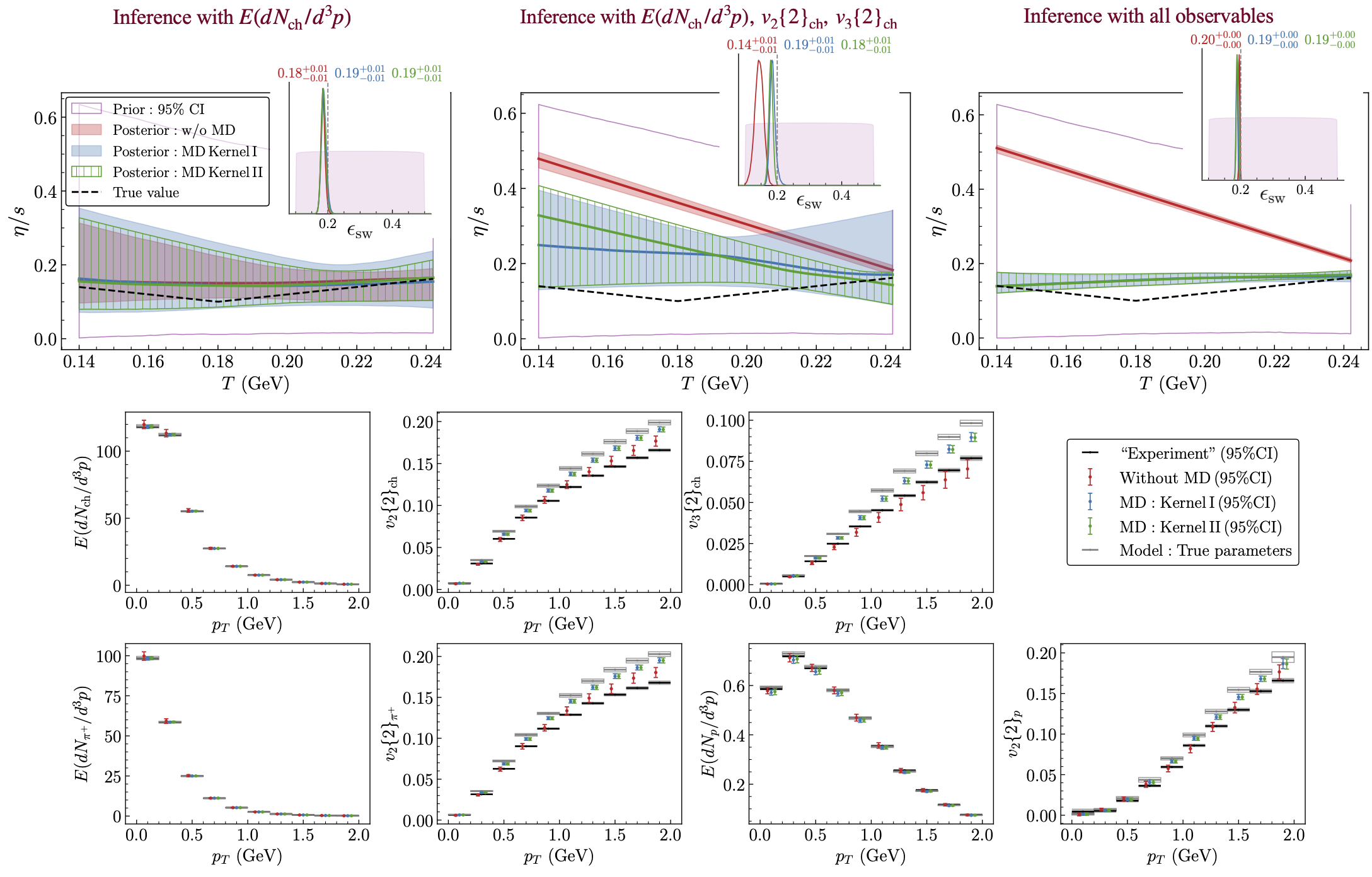
Fig. 11.11 Results for the five-parameter hydrodynamic simulation with parametrized \(\eta/s\) using mock data generated using a parametrization of \(\eta/s\) with \(T_{\rm kink}{\,=\,}0.18\,{\rm GeV}\), \(a_{\rm low}{\,=\,}{-}1\,{\rm GeV}^{-1}\), \(a_{\rm high}{\,=\,}1\,{\rm GeV}^{-1}\), and \((\eta/s)_{\rm kink}{\,=\,}0.1\), along with \(\epsilon_{\rm sw}{\,=\,}0.2\,\)GeV/fm\(^3\). The plot layouts and legends are identical to those in the previous figure. The corner plot for all five model parameters, when all available observables are included, is provided below.

The results in Fig. 11.11 support the overall conclusions drawn from the preceding cases: inference including the MD term performs significantly better than inference without MD. Still, we observe that in this last example none of the cases (with or without accounting for MD) accurately captures the shape of \((\eta/s)(T)\). We suspect that the available data do not provide sufficient information to properly constrain it given the theoretical deficiencies (i.e. the neglect of viscous corrections in the particlization routine) of the model. Even with MD, simply knowing that the model is more reliable at small \(p_T\) than at large \(p_T\) is not enough to resolve the shape of \((\eta/s)(T)\). Nonetheless, the improvement over conventional Bayesian fits remains substantial.

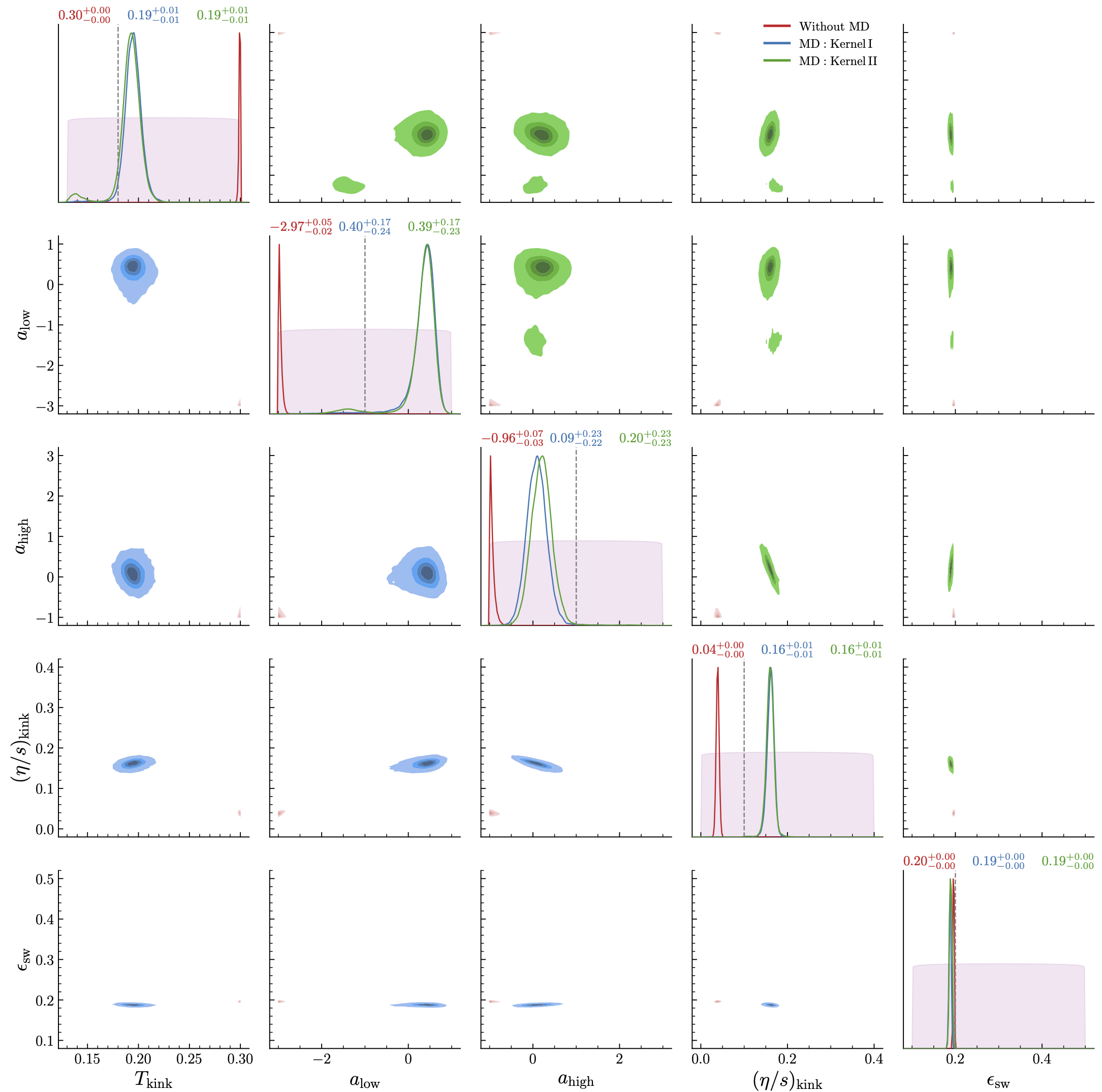
Fig. 11.12 Corner plot of all model parameters (with median \(\pm 68\%\) CI displayed on the diagonals) for the five-parameter model with parametrized \(\eta/s\), using mock data generated via the parametrization with \(T_{\rm kink}=0.18\,{\rm GeV}\), \(a_{\rm low}=-1\), \(a_{\rm high}=1\), and \((\eta/s)_{\rm kink}=0.1\), along with \(\epsilon_{\rm sw}=0.2\,\)GeV/fm\(^3\). This plot corresponds to the results shown in Fig. 11.11.

Overall better agreement with the true values is observed when the model discrepancy (MD) term is included (blue, green) compared to the no-MD case (red). The inability of the posteriors to accurately capture the slopes \(a_{\rm low}\) and \(a_{\rm high}\) is reflected in the nearly flat shape of \(\eta/s\) as a function of temperature in Fig. 11.11 for the MD cases. We observe that the absence of increasing specific viscosity on either side of \(T_{\rm kink}\), as seen in the truth, is compensated by an overestimated posterior for \((\eta/s)_{\rm kink}\) (for blue, green). We attribute the framework’s inability to accurately capture the posteriors for these parameters to a combination of limitations in the theoretical model, insufficient information in data to constrain the slopes, and weak prior information regarding the model’s domain used in the kernel modeling.

Phenomenological constraints on QCD transport with quantified theory uncertainties

Sunil Jaiswal, arXiv:2509.19759.

Abstract: We present data-driven, state-of-the-art constraints on the temperature-dependent specific shear and bulk viscosities of the quark–gluon plasma from Pb–Pb collisions at \(\sqrt{s_{\text{NN}}}\) = 2.76 TeV. We perform global Bayesian calibration using the JETSCAPE multistage framework with two particlization ansatze, Grad 14-moment and first-order Chapman–Enskog, and quantify theoretical uncertainties via a centrality-dependent model discrepancy term. When theoretical uncertainties are neglected, the specific bulk viscosity and some model parameters inferred using the two ans¨atze exhibit clear tension. Once theoretical uncertainties are quantified, the Grad and Chapman-Enskog posteriors for all model parameters become almost statistically indistinguishable and yield reliable, uncertainty-aware constraints. Furthermore, the learned discrepancy identifies where each model falls short for specific observables and centrality classes, providing insight into model limitations.

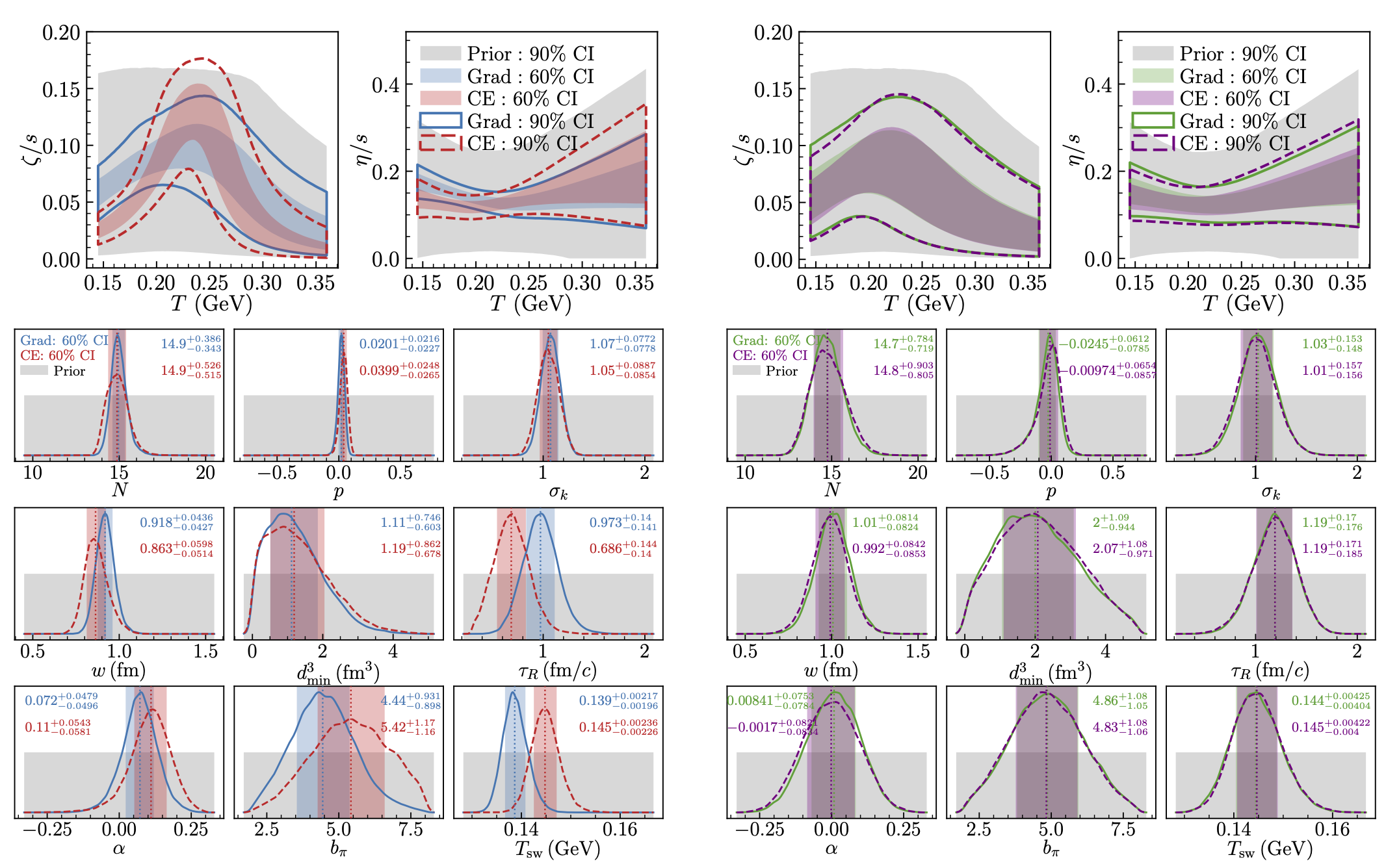
Fig. 11.13 Left: Parameter inference without accounting for theoretical uncertainty (w/o MD). Top row: Posteriors for the specific bulk and shear viscosities, with central 90% and 60% credible interval (CI) bands. The shaded gray regions denote the 90% prior intervals. Bottom rows: Solid and dashed curves show the posterior distributions for the remaining model parameters. Colored shaded regions show the central 60% CI, and shaded gray regions indicate the uniform prior range. In each subplot, a dotted vertical line marks the posterior median, and the printed value reports median \(\pm60\%\) CI. Right: Parameter inference accounting for theoretical uncertainty (w/ MD) with the same layouts and legends as on the left.

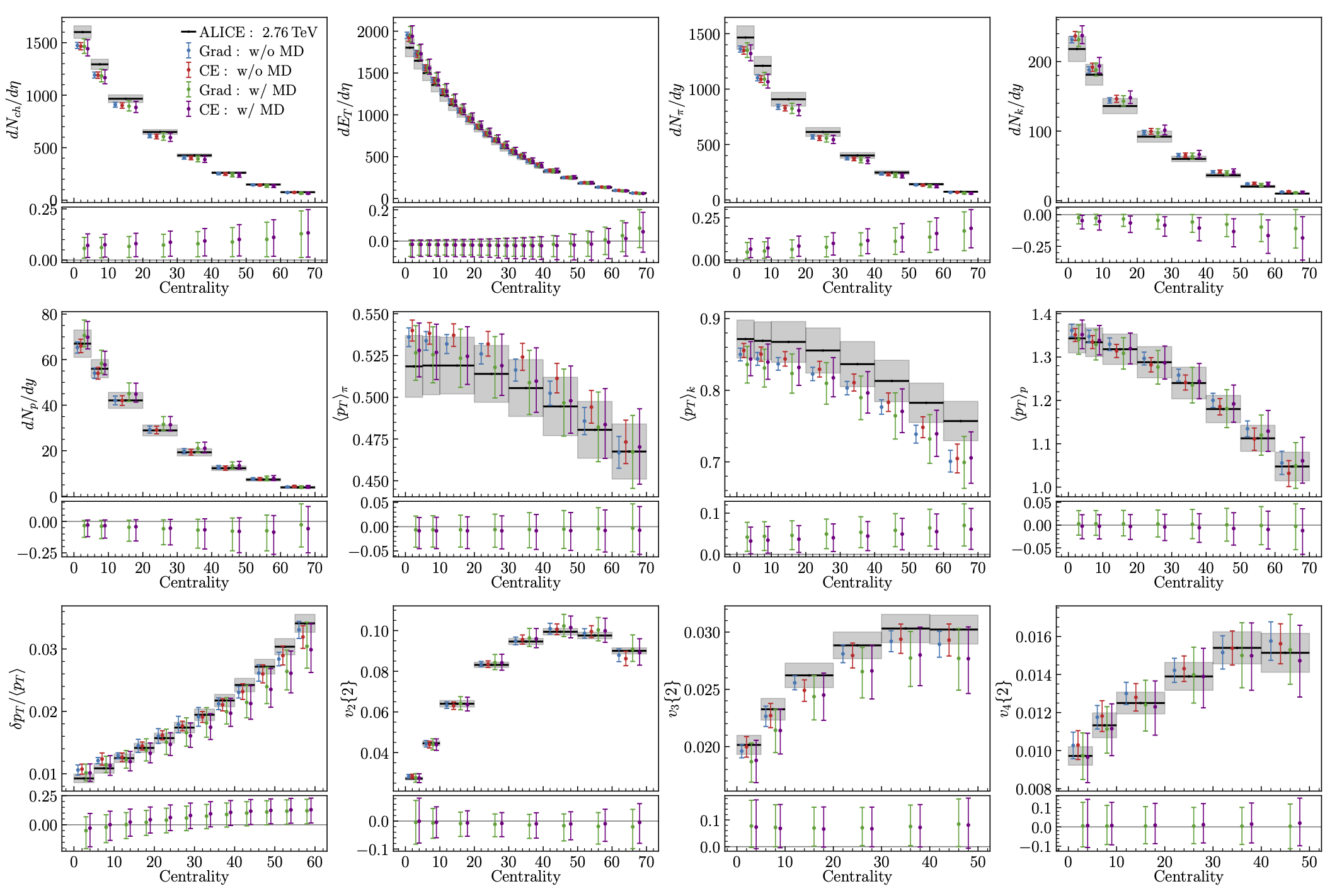
Fig. 11.14 Model predictions, obtained using the parameter posteriors shown above, are compared with ALICE data (black). Panels below each observable show the normalized model discrepancies from the w/ MD predictions.

Summary: Model–to-data comparison requires careful quantification of both experimental and theoretical uncertainties. Theoretical models have inherent limitations, and using them beyond their domains of validity without accounting for theory error can bias parameter estimates, reducing model parameters to mere fitting variables. In this work, we employ a Bayesian framework that quantifies theoretical uncertainties to constrain the temperature-dependent shear and bulk viscosities of the quark-gluon plasma from Pb–Pb collision data at \(\sqrt{s_{\text{NN}}}\) = 2.76 TeV. We show that, without accounting for theory errors, the multistage JETSCAPE framework with Grad and Chapman–Enskog particlization leads to tensions in the inferred transport coefficients and model parameters. Once the theoretical uncertainties are quantified, these tensions disappear and the Grad and CE posteriors become statistically indistinguishable across all shared parameters. This collapse of the model dependence yields reliable constraints on QGP viscosities in the temperature range \(T \sim\) 150-350 MeV, where first-principles calculations remain limited. The learned discrepancy further provides insight into the limitations of the theoretical models.