
31.2. Bayesian inference for network weights#
A Bayesian neural network can be viewed as probabilistic model in which we want to infer \(p(y \lvert \boldsymbol{x},\mathcal{D})\) where \(\mathcal{D} = \left\{\boldsymbol{x}^{(i)}, y^{(i)}\right\}\) is a given training dataset.
Maximum likelihood and MAP estimates#
We construct the likelihood function \(p(\mathcal{D} \lvert \boldsymbol{w}) = \prod_i p(y^{(i)} \lvert \boldsymbol{x}^{(i)}, \boldsymbol{w})\) which is a function of parameters \(\boldsymbol{w}\). Maximizing the likelihood function gives the maximum likelihood estimate (MLE) of \(\boldsymbol{w}\). The usual optimization objective during training is the negative log likelihood. For a categorical distribution this is the cross entropy error function, for a Gaussian distribution this is proportional to the sum of squares error function. MLE can lead to severe overfitting though.
Multiplying the likelihood with a prior distribution \(p(\boldsymbol{w})\) is, by Bayes theorem, proportional to the posterior distribution \(p(\boldsymbol{w} \lvert \mathcal{D}) \propto p(\mathcal{D} \lvert \boldsymbol{w}) p(\boldsymbol{w})\). Maximizing \(p(\mathcal{D} \lvert \boldsymbol{w}) p(\boldsymbol{w})\) gives the maximum a posteriori (MAP) estimate of \(\boldsymbol{w}\). Computing the MAP estimate has a regularizing effect and can prevent overfitting. The optimization objectives here are the same as for MLE plus a regularization term coming from the log prior.
The posterior predictive distribution#
Both MLE and MAP give point estimates of parameters. If we instead had a full posterior distribution over parameters we could make predictions that take weight uncertainty into account. This is covered by the posterior predictive distribution \(p(y \lvert \boldsymbol{x},\mathcal{D}) = \int p(y \lvert \boldsymbol{x}, \boldsymbol{w}) p(\boldsymbol{w} \lvert \mathcal{D}) d\boldsymbol{w}\) in which the parameters have been marginalized out. This is equivalent to averaging predictions from an ensemble of neural networks weighted by the posterior probabilities of their parameters \(\boldsymbol{w}\).
Returning to the binary classification problem, \(y^{(n+1)}\) corresponds to the probability \(p_{t^{(n+1)}=1}\) and a Bayesian prediction of a new datum \(y^{(n+1)}\) will correspond to a pdf and involves marginalizing over the weight and bias parameters
where we have also included the weight decay hyperparameter \(\alpha\) from the prior (regularizer). Marginalization could, of course, also be performed over this parameter.
Example: the Bayesian binary classifier#
We show an example of such inference, comparing the point estimate \(y(x; w^*, \alpha)\) and the Bayesian approach, in Fig. 31.2.
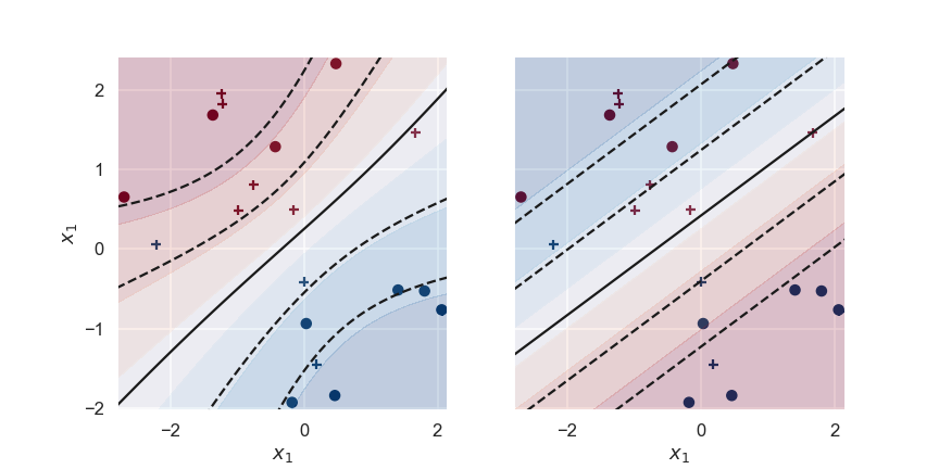
Fig. 31.2 The predictions for a Bayesian (left panel) and regular (right panel) binary classifier that has been learning from ten training data (circles) with a weight decay \(\alpha = 1.0\). The decision boundary (\(y=0.5\), i.e. the activation \(a=0\)) is shown together with the levels 0.12,0.27,0.73,0.88 (corresponding to the activation \(a=\pm1,\pm2\)). Test data is shown as plus symbols.#
The Bayesian classifier is based on sampling a very large ensemble of single neurons with different parameters. The distribution of these samples will be proportional to the posterior pdf for the parameters. The decision boundary shown in the figure is obtained as the mean of the predictions of the sampled neurons evaluated on a grid. It is clear that the Bayesian classifier is more uncertain about its predictions in the lower left and upper right corners, where there is little training data.
This becomes even more clear when we plot the standard deviation of the predictions of the Bayesian classifier in Fig. 31.3.
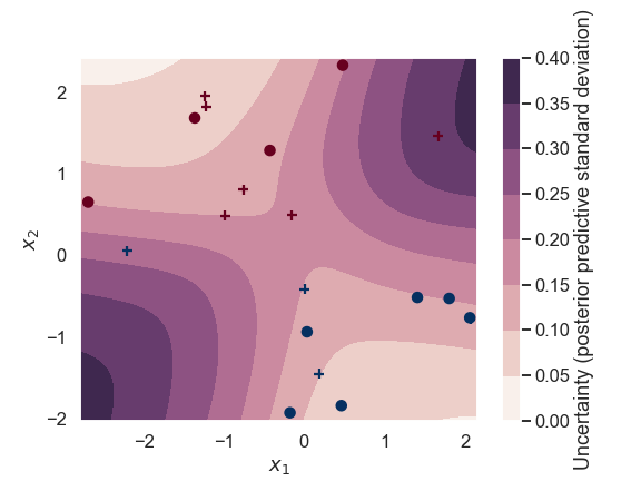
Fig. 31.3 The standard deviation of the class label predictions for a Bayesian binary classifier.#
The predictions are rather certain along a diagonal line (close to the training data). Note that the interpretation of the prediction in the center of Fig. 31.3 (near \(x_1,x_2 = 0,0\)) is the following: The Bayesian binary classifier predicts a probability of \(\sim 0.5\) for this point in the input parameter space to belong to class 1 (i.e. the decision is very uncertain). The Bayesian classifier is also very certain about this uncertainty (the standard deviation is small).
In contrast, predictions for points in the upper left or lower right corners are very certain about the class label (and there is little uncertainty about this certainty).
This is the distinction of Probabilistic neural network made concrete. The value \(y \approx 0.5\) at the centre is aleatoric: even with the weights known exactly, the label of a point sitting on the decision boundary is a coin toss, and no amount of further training data would change that. The spread of \(y\) across the sampled weights is epistemic: it measures how much the classifier’s opinion depends on which weights we happen to draw, and it shrinks wherever the training data pin the boundary down. The two figures show that the two are independent of each other. Near the origin the aleatoric uncertainty is at its largest while the epistemic uncertainty is small; in the upper left and lower right corners it is the other way round. That is precisely why they are worth reporting separately: they answer different questions, and only one of them would be reduced by collecting more data.
Note also that the aleatoric part required no extra machinery here. The output \(y\) is the parameter of a Bernoulli distribution, so it carries its own width. In a Bayesian neural network approach to a regression problem this is no longer the case. The width has to be supplied explicitly, either as a fixed number or as a further output of the network.