
31.1. Probabilistic neural network#
We use \(y\) to denote the output from the neural network. This output could, in general, be a vector. The neural network can therefore be seen as a non-linear mapping \(y(\boldsymbol{x}; \boldsymbol{w})\): \(x \in \mathbb{R}^p \to y \in \mathbb{R}^m\). The training of the network implies feeding it with training data and finding the sets of weights and biases that minimizes a loss function that has been selected for that particular problem. We will now be interested in probabilistic machine-learning models for which predictions are represented by probability distributions.
A Bayesian binary classifier#
Consider first a classification problem where the single output \(y\) of the final network layer is a real number \(\in [0,1]\) that indicates the (discrete) probability for input \(\boldsymbol{x}\) belonging to either class \(t=1\) or \(t=0\):
The output \(y\) is in fact the parameter of a Bernoulli distribution over \(t\). For a classification task, an optimized-weights network with a single output therefore delivers a complete probability distribution for the datum. The distribution width, \(y(1-y)\), is already built in. For a regression problem, a probabilistic model might need to output more than one parameter to specify probability distributions for target data. We return to this in Bayesian neural networks in practice.
A simple binary classifier can be trained by minimizing the loss function
made up of an error function
where \(t^{(n)}\) is the training data, and the regularizer
is designed to avoid overfitting. The error function can be interpreted as minus the log likelihood, with the likelihood
Similarly the regularizer can be interpreted in terms of a log prior probability distribution over the parameters. With the quadratic \(E_W\) given above, the corresponding prior distribution is a Gaussian with variance \(\sigma_W^2 = 1/\alpha\) and \(1/Z_W = (\alpha/2\pi)^{K/2}\), where \(K\) is the number of parameters in \(w\).
The objective function \(C_W(w)\) then corresponds to a (unnormalized) negative log-posterior for the parameters \(\boldsymbol{w}\) given the data
We show the evolution of this probability distribution for a sequence of an increasing number of training data (\(N\)) in Fig. 31.1. The targets are either 0 or 1, as indicated by red and blue markers. The network parameters \(\boldsymbol{w}\) that are found by minimizing \(C_W(\boldsymbol{w})\) can be interpreted as the most probable parameter vector \(\boldsymbol{w}^*\).
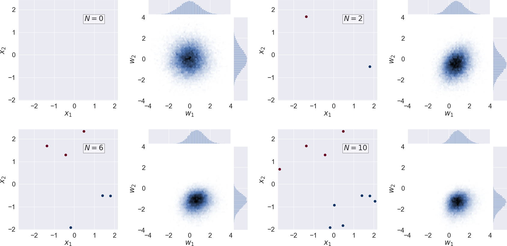
Fig. 31.1 Scatter plot of training data and the corresponding bivariate posterior PDF for the neuron weights \(p(w_1, w_2 | \mathcal{D}, \alpha)\) (i.e. marginalized over the bias \(w_0\)) for a sequence of \(N=0,2,6,10\) training data.#
Types of uncertainty#
In the following, we will use the full Bayesian approach and consider the information that is contained in the actual probability distribution. In fact, there are different types of uncertainty that will be addressed:
Epistemic uncertainties
correspond to what we do not know about the model, such as the “true” values of model parameters and, more drastically, whether the model class is able to represent the truth at all. The defining property is that this uncertainty is reduced by more data of the same kind. More training data narrows the posterior for the weights.
Aleatoric uncertainties
appear as a result of inherent noise in the data. They enter through the likelihood function and are therefore part of the Bayesian treatment from the start. The defining property is that this uncertainty cannot be reduced with more data of the same quality. More measurements pin down the size of the scatter more precisely, but the scatter itself remains. Aleatoric is derived from the Latin alea or dice, referring to a game of chance.
The machine-learning literature works with this two-way split of uncertainty in which model discrepancy, that we have discussed extensively in the context of scientific modeling, has no slot of its own. Conceptually it belongs with the epistemic uncertainties, since it is a statement about the model rather than about the data. Operationally, however, it is almost always absorbed into the aleatoric term. A network that reports a predictive uncertainty width will fit that width to whatever residual scatter remains. Such a machine-learning model has no way of telling whether the scatter comes from noise in the data or from its own inability to follow them. Obviously, it is worth knowing which type of uncertainty you are looking at, because the remedies differ — more data, a better measurement instrument, or a better model.
what the uncertainty is about |
reduced by more data of the same kind? |
usual label in the ML literature |
|
|---|---|---|---|
Parameter uncertainty |
our incomplete knowledge of the parameters \(\boldsymbol{w}\) |
yes |
epistemic |
Model discrepancy |
the model class not containing the truth |
no — only a better model helps |
see above |
Observational noise |
randomness in the measurement process itself |
no |
aleatoric |
This is also why the physicist’s statistical and systematic errors do not map onto the two labels. A statistical experimental error is aleatoric. A systematic experimental error, such as a calibration offset, is not reduced by repeating the measurement, but it is reducible by a better calibration. It is epistemic in the sense used here. Model discrepancy, meanwhile, is systematic in origin yet turns up in the aleatoric slot. The aleatoric/epistemic distinction is a statement about what more data of the same kind can fix; it is not a relabelling of statistical and systematic.