26.2. Binary classification

Let us specialize to the case of two classes only, with outputs \(t^{(i)} \in \{0,1\}\). That is

(26.1)\[\begin{equation} t^{(i)} = \begin{bmatrix} 0 \\ 1 \end{bmatrix} = \begin{bmatrix} \mathrm{no}\\ \mathrm{yes} \end{bmatrix}. \end{equation}\]

The perceptron

Before moving to the logistic model, let us try to use a linear regression model to classify these two outcomes. We could use a linear model

(26.2)\[\begin{equation} \boldsymbol{\tilde{y}} = \boldsymbol{X} \boldsymbol{w}, \end{equation}\]

where \(\boldsymbol{\tilde{y}}\) is a vector representing the possible outcomes, \(\boldsymbol{X}\) is our \(n\times p\) design matrix and \(\boldsymbol{w}\) are the model parameters.

Note however that our outputs \(\tilde{y}^{(i)} \in \mathbb{R}\) take values on the entire real axis. Our targets \(t^{(i)}\), however, are discrete variables.

One simple way to get a discrete output is to have sign functions that map the output of a linear regressor to values \(y^{(i)} \in \{ 0, 1 \}\), \(y^{(i)} = f(\tilde{y}^{(i)})=\frac{\mathrm{sign}(\tilde{y}^{(i)})+1}{2}\), which will map to one if \(\tilde{y}^{(i)}\ge 0\) and zero otherwise. Historically this model is called the perceptron in the machine learning literature.

The perceptron is an example of a “hard classification” model. We will encounter this model when we discuss neural networks as well. Each datapoint is deterministically assigned to a category (i.e \(y^{(i)}=0\) or \(y^{(i)}=1\)). In many cases, it is favorable to have a soft classifier that outputs the probability of a given category rather than a single value. For example, given \(\boldsymbol{x}^{(i)}\), the classifier outputs the probability of being in a category \(k\).

The logistic function

Logistic regression is the simplest example of the use of such a soft classifier. Let us assume that we have two classes such that \(t^{(i)}\) is either \(0\) or \(1\).

In logistic regression, we will use the so-called logit function

(26.3)\[\begin{equation} y(\boldsymbol{x}; \boldsymbol{w}) = y(z) = \frac{1}{1+e^{-z}} = \frac{e^z}{1+e^z}, \end{equation}\]

with the so called activation \(z = z(\boldsymbol{x}; \boldsymbol{w})\). This function is no longer linear in the model parameters \(\boldsymbol{w}\). It is an example of a S-shape or Sigmoid function.

We let \(y^{(i)}\) give the probability that a data point \(\boldsymbol{x}^{(i)}\) belongs to category \(t^{(i)} = 1\),

(26.4)\[\begin{equation} \prob \left( t^{(i)} = 1 \vert \boldsymbol{x}^{(i)}, \boldsymbol{w} \right) = y(\boldsymbol{x}^{(i)}; \boldsymbol{w}). \end{equation}\]

• Most frequently one uses \(z = z(\boldsymbol{x}, \boldsymbol{w}) \equiv \boldsymbol{x} \cdot \boldsymbol{w}\).

• It is common to introduce also a bias, or threshold, weight \(w_0\). This can be accommodated by prepending a constant feature \(x_0^{(i)}=1\) for all \(i\).

• Note that \(1-y(z)= y(-z)\).

• The sigmoid function can be motivated in several different ways:

  • In information theory this function represents the probability of a signal \(s=1\) rather than \(s=0\) when transmission occurs over a noisy channel.

  • It can be seen as an artificial neuron that mimics aspects of its biological counterpart.

Standard activation functions

Show code cell content

Hide code cell content

import numpy as np
import matplotlib.pyplot as plt
from myst_nb import glue

# Set the relevant activation interval 
z = np.linspace(-6,6,num=1201)

# Perceptron model
def y_perceptron(z):
    return (np.sign(z)+1)/2
    
# logit model
def y_logit(z):
    return 1 / (1+np.exp(-z))
    
# tanh model
def y_tanh(x):
    return (np.tanh(z)+1)/2
    
    
# Create a visualization
fig, ax = plt.subplots(nrows=1, ncols=1, sharey=True, **{"figsize":(6,4)})
ax.plot(z,y_perceptron(z),label='perceptron',lw=2,ls='-.',color='red')
ax.plot(z,y_logit(z),label='logit',lw=2,ls='-',color='blue')
ax.plot(z,y_tanh(z),label='tanh (normalized)',lw=2,ls='--',color='black')
ax.legend(loc='best')
ax.set_xlabel(r'Activation $z$')
ax.set_ylabel('Activation function')

glue("sigmoid_functions_fig", fig, display=False)

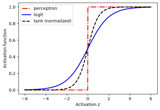
Fig. 26.1 The sigmoid, step,and (normalized) tanh functions; three common classifier functions used in classification and neural networks. In these lecture notes we use the letter \(z\) to denote the activation.

A binary classifier with two parameters

We assume now that we have two classes with \(t^{(i)}\) being either \(0\) or \(1\). Furthermore we assume also that we have only two parameters \(w_0, w_1\) and the features \(\boldsymbol{x}^{(i)} = \{ 1, x^{(i)} \}\) defining the activation function. I.e., there is a single independent (input) variable \(x\). We can produce probabilities from the classifier output \(y^{(i)}\)

\[\begin{align*} \prob (t^{(i)}=1|x^{(i)},\boldsymbol{w}) &= y(z^{(i)})= \frac{\exp{(w_0+w_1x^{(i)})}}{1+\exp{(w_0+w_1x^{(i)})}},\\ \prob (t^{(i)}=0|x^{(i)},\boldsymbol{w}) &= 1 - \prob (t^{(i)}=1|x^{(i)},\boldsymbol{w}) = \frac{1}{1+\exp{(w_0+w_1x^{(i)})}}, \end{align*}\]

where \(\boldsymbol{w} = ( w_0, w_1)\) are the weights we wish to extract from training data.

Determination of weights

Among ML practitioners, the prevalent approach to determine the weights in the activation function(s) is by minimizing some kind of cost function using some version of gradient descent. As we will see this usually corresponds to maximizing a likelihood function with or without a regularizer.

In this course we will obviously also advocate (or at least make aware of) the more probabilistic approach to learning about these parameters.

Maximum likelihood

In order to define the total likelihood for all possible outcomes from a dataset \(\mathcal{D}=\{(x^{(i)}, t^{(i)},)\}\), with the binary labels \(t^{(i)}\in\{0,1\}\) and where the data points are drawn independently, we use the binary version of the Maximum Likelihood Estimation (MLE) principle. We express the likelihood in terms of the product of the individual probabilities of a specific outcome \(t^{(i)}\), that is

\[\begin{align*} \mathcal{L} = \prob (\mathcal{D}|\boldsymbol{w})& = \prod_{i=1}^N \left[p(t^{(i)}=1|x^{(i)},\boldsymbol{w})\right]^{t^{(i)}}\left[1-p(t^{(i)}=1|x^{(i)},\boldsymbol{w}))\right]^{1-t^{(i)}}\nonumber \\ \end{align*}\]

The cost/loss function (to be minimized) is then defined as the negative log-likelihood

(26.5)\[\begin{equation} \mathcal{C}(\boldsymbol{w}) = -L \equiv -\log(\mathcal{L}) = -\sum_{i=1}^N \left( t^{(i)}\log{\prob (t^{(i)}=1|x^{(i)},\boldsymbol{w})} + (1-t^{(i)})\log\left[1-\prob (t^{(i)}=1|x^{(i)},\boldsymbol{w}))\right]\right). \end{equation}\]

The cost function rewritten as cross entropy

Using the definitions of the probabilities we can rewrite the cost/loss function as

(26.6)\[\begin{equation} \mathcal{C}(\boldsymbol{w}) = -\sum_{i=1}^N \left( t^{(i)}\log{ y(x^{(i)},\boldsymbol{w})} + (1-t^{(i)})\log\left[ 1-y( x^{(i)},\boldsymbol{w}) \right] \right), \end{equation}\]

which can be recognised as the relative entropy between the empirical probability distribution \((t^{(i)}, 1-t^{(i)})\) and the probability distribution predicted by the classifier \((y^{(i)}, 1-y^{(i)})\). Therefore, this cost function is known in statistics as the cross entropy.

Using specifically the logistic sigmoid activation function with two weights, and reordering the logarithms, we can rewrite the log-likelihood to obtain

(26.7)\[\begin{equation} \mathcal{C}(\boldsymbol{w})=-\sum_{i=1}^N \left[ t^{(i)} (w_0+w_1x^{(i)}) -\log{ \left( 1+\exp{(w_0+w_1x^{(i)})} \right) } \right]. \end{equation}\]

MLE should give the weights \(\boldsymbol{w}^*\) that minimizes this cost function.

Regularization

In practice, just as for linear regression, one often supplements the cross-entropy cost function with additional regularization terms, usually \(L_1\) and \(L_2\) regularization. This introduces hyperparameters into the classifier.

In particular, Ridge regularization is obtained by defining another cost function

(26.8)\[\begin{equation} \mathcal{C}_W (\boldsymbol{w}) \equiv \mathcal{C} (\boldsymbol{w}) + \alpha E_W (\boldsymbol{w}) \end{equation}\]

where \(E_W (\boldsymbol{w}) = \frac{1}{2} \sum_j w_j^2\) and \(\alpha\) is known as the weight decay.

Question

Can you motivate why \(\alpha\) is known as the weight decay?

Hint: Recall the origin of this regularizer from a Bayesian perspective.

Minimizing the cross entropy

The cross entropy is a convex function of the weights \(\boldsymbol{w}\) and, therefore, any local minimizer is a global minimizer.

Minimizing this cost function (here without regularization term) with respect to the two parameters \(w_0\) and \(w_1\) we obtain

\[\begin{align*} \frac{\partial \mathcal{C}(\boldsymbol{w})}{\partial w_0} &= -\sum_{i=1}^N \left(t^{(i)} -\frac{\exp{(w_0+w_1x^{(i)})}}{1+\exp{(w_0+w_1x^{(i)})}}\right) &= -\sum_{i=1}^N \left(t^{(i)} - y^{(i)} \right), \\ \frac{\partial \mathcal{C}(\boldsymbol{w})}{\partial w_1} &= -\sum_{i=1}^N \left(t^{(i)} x^{(i)} -x^{(i)}\frac{\exp{(w_0+w_1x^{(i)})}}{1+\exp{(w_0+w_1x^{(i)})}}\right) &= -\sum_{i=1}^N x^{(i)} \left(t^{(i)} - y^{(i)} \right). \end{align*}\]

A more compact expression

Let us now define a vector \(\boldsymbol{t}\) with \(n\) elements \(t^{(i)}\), an \(N\times 2\) matrix \(\boldsymbol{X}\) which contains the \((1, x^{(i)})\) predictor variables, and a vector \(\boldsymbol{y}\) of the outputs \(y^{(i)} = y(x^{(i)},\boldsymbol{w})\). We can then express the first derivative of the cost function in matrix form

(26.9)\[\begin{equation} \frac{\partial \mathcal{C}(\boldsymbol{w})}{\partial \boldsymbol{w}} = -\boldsymbol{X}^T\left( \boldsymbol{t}-\boldsymbol{y} \right). \end{equation}\]

A learning algorithm

Notice. Having access to the first derivative we can define an on-line learning rule as follows:

• For each input \(i\) (possibly permuting the sequence in each epoch) compute the error \(e^{(i)} = t^{(i)} - y^{(i)}\).

• Adjust the weights in a direction that would reduce this error: \(\Delta w_j = \eta e^{(i)} x_j^{(i)}\). The parameter \(\eta\) is called the learning rate.

• Perform multiple passes through the data, where each pass is known as an epoch. The computation of outputs \(\boldsymbol{y}\) given a set of weights \(\boldsymbol{w}\) is known as a forward pass, while the computation of gradients and adjustment of weights is called back-propagation.

You will recognise this learning algorithm as stochastic gradient descent.

Alternatively, one can perform batch learning for which multiple instances are combined into a batch, and the weights are adjusted following the matrix expression stated above. At the end, one hopes to have reached an optimal set of weights.

Extending to more features

Within a binary classification problem, we can easily expand our model to include multiple input features. Our activation function is then (with \(p\) features)

(26.10)\[\begin{equation} z( \boldsymbol{x}^{(i)}, \boldsymbol{w} ) = w_0 + w_1 x_1^{(i)} + w_2 x_2^{(i)} + \dots + w_p x_p^{(i)}. \end{equation}\]

Defining \(\boldsymbol{x}^{(i)} \equiv [1,x_1^{(i)}, x_2^{(i)}, \dots, x_p^{(i)}]\) and \(\boldsymbol{w}=[w_0, w_1, \dots, w_p]\) we get

(26.11)\[\begin{equation} \prob (t^{(i)}=1 | \boldsymbol{w}, \boldsymbol{x}^{(i)}) = \frac{ \exp{ \left( \boldsymbol{w} \cdot \boldsymbol{x}^{(i)} \right) }}{ 1 + \exp{ \left( \boldsymbol{w} \cdot \boldsymbol{x}^{(i)} \right) } }. \end{equation}\]