31.1. Basic neural network

We will consider a neuron with a vector of \(I\) input signals \(\boldsymbol{x} = \left\{ \boldsymbol{x}^{(i)} \right\}_{i=1}^I\), and an output signal \(y^{(i)}\), which is given by the non-linear function \(y(z)\) of the activation

(31.1)\[\begin{equation} z = w_0 + \sum_{i=1}^I w_i x_i, \end{equation}\]

where \(\boldsymbol{w} = \left\{ w_i \right\}_{i=1}^I\) are the weights of the neuron and we have included a bias (\(b \equiv w_0\)).

The training of the network implies feeding it with training data and finding the sets of weights and biases that minimizes a loss function that has been selected for that particular problem. Consider, e.g., a classification problem where the single output \(y\) of the final network layer is a real number \(\in [0,1]\) that indicates the (discrete) probability for input \(\boldsymbol{x}\) belonging to either class \(t=1\) or \(t=0\):

(31.2)\[\begin{align} p_{t=1} \equiv p(t=1 | \boldsymbol{w},\boldsymbol{x}) &= y \\ p_{t=0} \equiv p(t=0 | \boldsymbol{w},\boldsymbol{x}) &= 1-y, \end{align}\]

A simple binary classifier can be trained by minimizing the loss function

(31.3)\[\begin{equation} C_W(\boldsymbol{w}) = C(\boldsymbol{w}) + \alpha E_W(\boldsymbol{w}), \end{equation}\]

made up of an error function

(31.4)\[\begin{equation} C(\boldsymbol{w}) = -\sum_n \left[ t^{(n)} \log ( y(\boldsymbol{x}^{(n)},\boldsymbol{w})) + (1 - t^{(n)}) \log (1 - y(\boldsymbol{x}^{(n)},\boldsymbol{w})) \right], \end{equation}\]

where \(t^{(n)}\) is the training data, and the regularizer

(31.5)\[\begin{equation} E_W(\boldsymbol{w}) = \frac{1}{2} \sum_i w_i^2, \end{equation}\]

that is designed to avoid overfitting. The error function can be interpreted as minus the log likelihood, with the likelihood

(31.6)\[\begin{equation} p(\mathcal{D}|\boldsymbol{w}) \propto \exp\left[ - C(\boldsymbol{w}) \right]. \end{equation}\]

Similarly the regularizer can be interpreted in terms of a log prior probability distribution over the parameters. With the quadratic \(E_W\) given above, the corresponding prior distribution is a Gaussian with variance \(\sigma_W^2 = 1/\alpha\) and \(1/Z_W = (\alpha/2\pi)^{K/2}\), where \(K\) is the number of parameters in \(w\).

(31.7)\[\begin{equation} p(\boldsymbol{w} | \alpha) = \frac{1}{Z_W(\alpha)} \exp \left[ -\alpha E_W \right]. \end{equation}\]

The objective function \(C_W(w)\) then corresponds to the inference of the parameters \(\boldsymbol{w}\) given the data

(31.8)\[\begin{equation} p(\boldsymbol{w} | \mathcal{D}, \alpha) = \frac{p(D|\boldsymbol{w}) p(\boldsymbol{w}|\alpha)}{p(\mathcal{D}|\alpha)} = \frac{1}{Z_M} \exp [ -C_W(\boldsymbol{w}) ]. \end{equation}\]

We show the evolution of the probability distribution for a sequence of an increasing number of training data (\(N\)) in Fig. 31.1. The targets are either 0 or 1, as indicated by red and blue markers. The network parameters \(\boldsymbol{w}\) that are found by minimizing \(C_W(\boldsymbol{w})\) can be interpreted as the most probable parameter vector \(\boldsymbol{w}^*\).

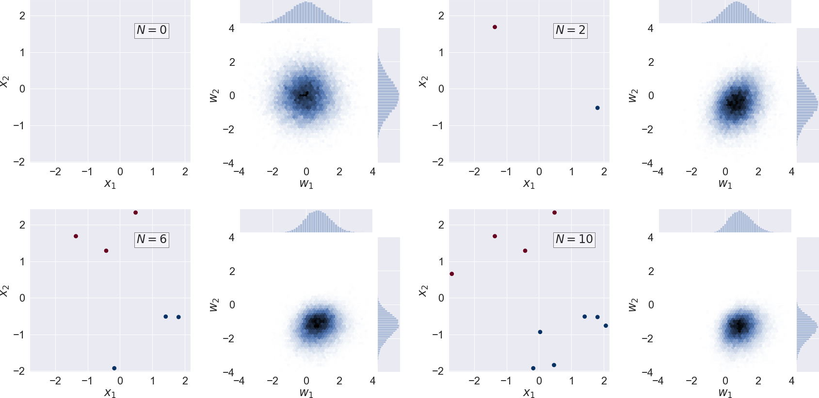
Fig. 31.1 Scatter plot of training data and the corresponding bivariate posterior pdf for the neuron weights \(p(w_1, w_2 | \mathcal{D}, \alpha)\) (i.e. marginalized over the bias \(w_0\)) for a sequence of \(N=0,2,6,10\) training data.

In the following, we will rather use the Bayesian approach and consider the information that is contained in the actual probability distribution. In fact, there are different uncertainties that should be addressed:

Epistemic uncertainties

correspond to uncertainties in the model. For a neural network we can learn about this uncertainty using test data. Epistemic uncertainty is also known as systematic uncertainty.

Aleatoric uncertainties

appear as a result of inherent noise in the training data. This should be included in the likelihood function (and is therefore part of the Bayesian approach). It can, however, not be reduced with more data of the same quality. Aleatoric uncertainty is also known as statistical uncertainty. Aleatoric is derived from the Latin alea or dice, referring to a game of chance.

Notice. We will use \(y\) to denote the output from the neural network. For classification problems, \(y\) will give the categorical (discrete) distribution of probabilities \(p_{t=c}\) of belonging to class \(c\). For regression problems, \(y\) is a continuous variable. It could also, in general, be a vector of outputs. The neural network can be seen as a non-linear mapping \(y(x; w)\): \(x \in \mathbb{R}^p \to y \in \mathbb{R}^m\).