27.2. Feed-forward networks: mathematical model

In this section we formulate the fully-connected feed-forward networks of Neural network types and architecture mathematically. We introduce the notation for signals, weights and biases that is used throughout the following sections, and the linear-algebra form that is used in practice.

Mathematical model

In a FFNN, the inputs to the nodes in one layer are the outputs of the nodes in the preceding layer.

Starting from the first hidden layer, we compute a weighted sum \(z_j^1\) of the input signals \(\boldsymbol{x} = (x_1, \ldots, x_n)\), for each node \(j\)

(27.2)\[\begin{equation} z_j^1 = \sum_{i=1}^{n} w_{ij}^1 x_i + b_j^1, \end{equation}\]

where \(w_{ij}^1\) are the linear weights of this node and \(b^1_j\) is known as a bias, or threshold, weight.

The value, \(z_j^1\), is known as the preactivation and becomes the argument to the activation function \(f^1(z)\) of node \(j\). For simplicity we assume that all nodes in one layer have the same activation function. The output from node \(j\) in the first layer then becomes

(27.3)\[\begin{equation} y_j^1 = f^1(z_j^1) = f^1\left(\sum_{i=1}^n w_{ij}^1 x_i + b_j^1\right). \label{outputLayer1} \end{equation}\]

When the output of all the nodes in the first hidden layer are computed, the preactivations of the subsequent layer can be calculated and so forth. Propagating signals from layer to layer we eventually reach node \(j\) in layer \(l\). Its output signal is produced via its activation function \(f^l(z^l_j)\)

(27.4)\[\begin{equation} y_j^l = f^l(z_j^l) = f^l\left(\sum_{i=1}^{N_{l-1}} w_{ij}^l y_i^{l-1} + b_j^l\right), \label{generalLayer} \end{equation}\]

where \(N_{l-1}\) is the number of nodes in layer \(l-1\).

The output layer of an \(L\)-layer network (i.e., with \(L-1\) hidden layers) is layer \(L\). For example, the final output from node \(i\) of a three-layer network reads

(27.5)\[\begin{equation} y^{3}_i = f^{3}\left[\sum_{k=1}^{N_2} w_{ki}^3 f^2 \left(\sum_{j=1}^{N_1}w_{jk}^{2} f^1\left(\sum_{n=1}^{N_0} w_{nj}^1 x_n+ b_j^1\right)+b_k^{2}\right)+b_i^3\right], \label{completeNN} \end{equation}\]

with \(N_0 = n\) the number of inputs. Deeper networks simply add further levels of nesting. This illustrates that the outputs \(\boldsymbol{y} = (y^{L}_1, \ldots, y^{L}_m)\) are the dependent variables and the input \(\boldsymbol{x}\) are the independent variables.

This confirms that a FFNN, despite its quite convoluted mathematical form, is nothing more than a non-linear mapping. For example it can map real-valued vectors \(\boldsymbol{x} \in \mathbb{R}^n \rightarrow \boldsymbol{y} \in \mathbb{R}^m\).

Furthermore, the flexibility and universality of a neural network can be illustrated by realizing that the expression is essentially a nested sum of scaled activation functions leading to

(27.6)\[\begin{equation} \boldsymbol{y} = \boldsymbol{y}(\boldsymbol{x}; \boldsymbol{W}), \end{equation}\]

where \(\boldsymbol{W}\) contains the weights and biases which are the model parameters.

Matrix-vector notation

We can introduce a much more convenient matrix-vector notation for all quantities in a FFNN.

In particular, we represent all signals as layer-wise row vectors \(\boldsymbol{y}^l\) so that the \(i\)-th element of each vector is the output \(y_i^l\) of node \(i\) in layer \(l\).

We have that \(\boldsymbol{W}^l\) is an \(N_{l-1} \times N_l\) matrix, while \(\boldsymbol{b}^l\) and \(\boldsymbol{y}^l\) are \(1 \times N_l\) row vectors. With this notation, the sum becomes a matrix-vector multiplication, and we can write the preactivations of layer \(l\) as

(27.7)\[\begin{equation} \boldsymbol{z}^l = \boldsymbol{y}^{l-1} \boldsymbol{W}^l + \boldsymbol{b}^{l}, \end{equation}\]

where \(\boldsymbol{y}^0 \equiv \boldsymbol{x}\). The outputs of this layer then become \(\boldsymbol{y}^{l} = f^l(\boldsymbol{z}^{l})\), where we should understand element-wise application of the activation function.

For \(N\) data instances stacked as the rows of a matrix, the same expression reads \(\boldsymbol{Z}^l = \boldsymbol{Y}^{l-1} \boldsymbol{W}^l + \boldsymbol{b}^l\), with the bias added to each row. In code this is Y @ W + b, with Y = X for the first layer.

As an example we consider the outputs of the second layer. Assuming three nodes in the first layer we get

(27.8)\[\begin{equation} \boldsymbol{y}^2 = f^2(\boldsymbol{y}^{1} \boldsymbol{W}^2 + \boldsymbol{b}^{2}) = f^2\left( \left[ y^1_1, y^1_2, y^1_3 \right] \left[\begin{array}{ccc} w^2_{11} &w^2_{12} &w^2_{13} \\ w^2_{21} &w^2_{22} &w^2_{23} \\ w^2_{31} &w^2_{32} &w^2_{33} \\ \end{array} \right] + \left[ b^2_1, b^2_2, b^2_3 \right]\right). \end{equation}\]

This is not just a convenient and compact notation, but also a useful and intuitive way to think about FFNNs. The output is calculated by a sequence of matrix-vector multiplications and vector additions used as input to activation functions.

Activation rules

A property that characterizes a neural network, other than its connectivity, is the choice of activation function(s). In general, these are non-linear functions. In fact, a FFNN with only linear activation functions would imply that each layer simply performs a linear transformation of its inputs and the output would be an unnecessarily complicated linear mapping of the input.

Logistic and Hyperbolic activation functions. The archetypical example of activation functions is the family of S-shaped (sigmoid) functions. In particular, the logistic sigmoid function is

(27.9)\[\begin{equation} f_\mathrm{sigmoid}(z) = \frac{1}{1 + e^{-z}}, \end{equation}\]

and the hyperbolic tangent function is

(27.10)\[\begin{equation} f_\mathrm{tanh}(z) = \tanh(z) \end{equation}\]

Noisy networks

Both the sigmoid and tanh activation functions imply that signals will be non-zero everywhere. Even when nodes are inactive, they transmit small, but nonzero, signals. This leads to inefficiencies in both feed-forward and back-propagation operations.

The ambition to completely silence inactive neurons leads to the family of rectifier activation functions. The Rectifier Linear Unit (ReLU) uses the following activation function

(27.11)\[\begin{equation} f_\mathrm{ReLU}(z) = \max(0,z). \end{equation}\]

However, this type of activation function gives zero gradients, \(f'(z) = 0\) for \(z<0\), which makes weight updates during training much less efficient. To solve this problem, known as dying ReLU neurons, practitioners often use modified versions of the ReLU function, such as the leaky ReLU or the exponential linear unit (ELU) function

(27.12)\[\begin{equation} f_\mathrm{ELU}(z) = \left\{\begin{array}{cc} \alpha\left( \exp{(z)}-1\right) & z < 0,\\ z & z \ge 0.\end{array}\right. \end{equation}\]

The final layer of a neural network has to use an activation function that produces a relevant output signal for the task at hand. For example, the output nodes could employ a linear activation function to give continuous outputs for regression tasks, or a softmax function to provide classification probabilities.

Learning algorithm

The learning phase (network training) aims to optimize the weights to minimize a problem and data-specific cost function. This task involves multiple choices

1. Choosing a cost function, \(C(\trainingdata, \boldsymbol{W})\), that describes how to compare model outputs with targets from a training data set \(\trainingdata = \left\{ (\inputs_i, \targets_i) \right\}_{i=1}^{N}\). Each pair consists of an input \(\inputs_i\) and the target \(\targets_i\) that the network output \(\boldsymbol{y}(\inputs_i; \boldsymbol{W})\) should reproduce.

   • Common cost-function choices include: Mean-squared error (MSE) or Mean-absolute error (MAE) for regression; Cross-entropy or Accuracy for classification.

   • Weight regularization or random node dropout to avoid overfitting.

   • The incorporation of physics (model) knowledge in the construction of a more relevant cost function.

2. Optimization algorithm.

   • Back-propagation (see Neural networks: Backpropagation) can be used to compute the gradient of the cost function with respect to the weights. It corresponds to repeated use of the chain rule on the activation functions while traversing the different layers backwards.

   • The gradient evaluated after each parameter update can be used to iteratively search for a (local) optimum in the high-dimensional space of weights. Popular gradient descent optimizers include:

     • Standard stochastic gradient descent (SGD), possibly with batches.

     • Momentum SGD (to incorporate a moving average)

     • AdaGrad (with per-parameter learning rates)

     • RMSprop (adapting the learning rates based on RMS gradients)

     • Adam (a combination of momentum and RMSprop that employs estimates of both the first and second moments of weight gradients).

3. Splits of data

   • Training data: used for training.

   • Validation data: used to monitor learning and to adjust hyperparameters.

   • Test data: for final test of perfomance.

General remarks on training:

• It is critical that neither validation nor test data is used for adjusting the network weights.

• Data is often split into batches such that gradients are computed for a batch of data rather than for the full set all at once.

• A full pass of all data is known as an epoch. A validation score is often evaluated at the end of each epoch.

• Additional “hyperparameters” that can be tuned include:

  • The number of epochs (overfitting eventually).

  • The batch size (interplay between stochasticity and efficiency).

  • Learning rates.

In conclusion, there are many options when designing and training an neural network.

Exercises

Exercise 27.1 (Weights and signal propagation of a simple neural network)

Consider a neural network with two nodes in the input layer, one hidden layer with three nodes, and an output layer with one node (see Fig. 27.2). All active nodes (i.e., those that map input signals to an output via an activation function) employ the same activation function \(f(z) = 1 / (1 + e^{-z})\) and include a bias weight when computing the preactivation \(z\).

• a) How many free (trainable) parameters does this neural network have?

• b) Write an explicit expression for the output signal \(y\) from the output node as a function of its weights \((w^2_{11}, w^2_{12},w^2_{13})\), bias weight \(b^2_1\), and the signals \((y^1_1, y^1_2,y^1_3)\) coming from the nodes in the hidden layer.

• c) Write a vector expression for the preactivations \((z^1_1, z^1_2, z^1_3)\) of the three nodes in the hidden layer given a vector of inputs \((x_1, x_2)\) and a matrix that contains the weights of the hidden layer and a vector that contains the bias weights. Be explicit how the weights are ordered in the matrix such that the preactivation vector can be obtained with matrix-vector operations.

• d) How can the above expression be generalized to handle a scenario when there are four instances of input data?

\[\begin{split} \boldsymbol{X} = \begin{pmatrix} x^{(1)}_1 & x^{(1)}_2 \\ x^{(2)}_1 & x^{(2)}_2 \\ x^{(3)}_1 & x^{(3)}_2 \\ x^{(4)}_1 & x^{(4)}_2 \end{pmatrix} \end{split}\]

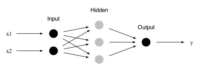
Fig. 27.2 A simple two-layer neural network.

Exercise 27.2 (Weights and signal propagation of a wide neural network)

Consider a neural network with three nodes in the input layer, one hidden layer with one hundred nodes, and an output layer with two nodes. All nodes in the hidden layer employ the same activation function \(f(z) = 1 / (1 + e^{-z})\) and include a bias weight when computing the preactivation \(z\). The nodes in the output layer are linear.

• a) How many free (trainable) parameters does this neural network have?

• b) Introduce relevant matrices and vectors to write down an expression for the output signal \(\boldsymbol{y} = (y_1, y_2)\) given an input \(\boldsymbol{x} = (x_1, x_2, x_3)\).

• c) How would this expression have to be modified to handle a scenario when there are \(N\) instances of input data, for which one would like to compute the corresponding network outputs?

Exercise 27.3 (Linear signals)

Consider a neural network with \(p\) nodes in the input layer, one hidden layer with \(L\) nodes, and an output layer with a single node. All nodes in the hidden layer employ the same activation function \(f(z) = 1 / (1 + e^{-z})\) and include a bias weight when computing the preactivation \(z\). The node in the output layer is linear.

• a) Consider small signals and weights such that the output from the nodes in the hidden layer can be approximated by linear functions in the input \(\inputs = (\inputt_1, \inputt_2, \ldots, \inputt_p)\). Write an expression for the output from one of these nodes.

• b) Show that the final output from the network also becomes linear in the inputs and relate the coefficients of this expression to the weights of the network.

Exercise 27.4 (Expected signal)

Consider a single node with \(p\) input signals, including a bias weight when computing the preactivation \(z\), and with a sigmoid activation function \(f(z) = 1 / (1 + e^{-z})\). All weights are initialized as independent draws from a standard normal distribution (zero mean and unit variance).

Assume that you would initialize a large number of instances of this kind of node. Each one will have different weights. For each one, you propagate the same input signal \(\inputs\) and measure the node’s preactivation \(z\) and output \(y\).

• a) How would the distribution \(\p{z}\) of the measured preactivations look like?

• b) How would the distribution \(\p{y}\) of the measured outputs look like?

• c) Study the form of \(\p{y}\) for the two different limits \(|\inputs| \ll 1\) (also with \(w_0 \ll 1\)) and \(|\inputs| \gg 1\).

Hints

You can choose to do task c) numerically, which is rather straightforward given that you have solved a) and b), or you can study it analytically which is straightforward for the first case (small signals) but harder for the second one.

For the numerical solution you might have problems with computer precision for large signals. You could consider rewriting your probability distribution, or just consider \(|\inputs| \approx 1\) is large enough to see the appearance of a bimodal distribution.

Solutions to exercises

Solution to Exercise 27.1 (Weights and signal propagation of a simple neural network)

• a) Trainable parameters are in the active nodes which, in this case, are the nodes in the hidden layer and the output layer. There are three weights per node in the hidden layer (two linear ones multiplying the two input signals and one bias) and four weights in the output node (three linear weights and one bias). Therefore, in total, there are \(3 \times 3 + 4 = 13\).

• b) \(y = 1 / (1+e^{-z})\), where \(z = w^2_{11} y^1_1 + w^2_{12} y^1_2 + w^2_{13} y^1_3 + b^2_1\).

• c) \(\boldsymbol{z}^{1} = \boldsymbol{x} \cdot \boldsymbol{W}^{1} + \boldsymbol{b}^{1}\), where \(\boldsymbol{z}^{1} = (z^1_1, z^1_2, z^1_3)\), \(\boldsymbol{x} = (x_1, x_2)\), \(\boldsymbol{b}^{1} = (b^1_1, b^1_2,b^1_3)\) are all row vectors and \(\boldsymbol{W}^{1} = \begin{pmatrix} w^{1}_{11} & w^{1}_{12} & w^{1}_{13} \\ w^{1}_{21} & w^{1}_{22} & w^{1}_{23} \end{pmatrix}\) is a \(2 \times 3\) matrix.

• d) It would look the same \(\boldsymbol{Z}^{1} = \boldsymbol{X} \cdot \boldsymbol{W}^{1} + \boldsymbol{b}^{1}\) but \(\boldsymbol{Z}^{1}\) would now be a \(4 \times 3\) matrix with each row containing the hidden layer node preactivations for the corresponding instance of input data (row in \(\boldsymbol{X}\)). Applying the activation function \(f(z)\) to each element of this matrix would give the corresponding output signals \(\boldsymbol{Y}^{1}\) as another \(4 \times 3\) matrix.

Solution to Exercise 27.2 (Weights and signal propagation of a wide neural network)

• a) There are \(100 \times (3+1) + 2 \times (100+1) = 602\) trainable parameters.

• b) \(\boldsymbol{y} = \boldsymbol{z} = \boldsymbol{y}^1 \boldsymbol{W}^2 + \boldsymbol{b}^2\), where the output layer parameters appear in the \(\boldsymbol{W}^2\) matrix and the \(\boldsymbol{b}^2\) vector.

  Furthermore, \(\boldsymbol{y}^1 = 1 / (1+e^{-\boldsymbol{z}^1})\) and \(\boldsymbol{z}^{1} = \boldsymbol{x} \boldsymbol{W}^{1} + \boldsymbol{b}^{1}\).

  The weight matrices and the bias vectors of layer \(L\) have elements \(w^L_{ij}\) and \(b^L_j\), respectively, and will have the sizes: \(\text{dim}(\boldsymbol{W}^{1}) = 3 \times 100\), \(\text{dim}(\boldsymbol{b}^{1}) = 1 \times 100\), \(\text{dim}(\boldsymbol{W}^{2}) = 100 \times 2\), \(\text{dim}(\boldsymbol{b}^{2}) = 1 \times 2\).

• c) In this case, the input, \(\boldsymbol{X}\), becomes an \(N \times 3\) matrix. The linear algebra expressions would look the same with the data instances representing one more dimension. That is \(\boldsymbol{Y} = \boldsymbol{Y}^1 \boldsymbol{W}^2 + \boldsymbol{b}^2\), with \(\text{dim}(\boldsymbol{Y}) = N \times 2\), and \(\boldsymbol{Y}^1 = f(\boldsymbol{Z}^1)\). Here, \(\boldsymbol{Z}^{1} = \boldsymbol{X} \boldsymbol{W}^{1} + \boldsymbol{b}^{1}\) is now an \(N \times 100\) matrix with each row containing the hidden layer node preactivations for the corresponding instance of input data (row in \(\boldsymbol{X}\)). Furthermore, signals \(\boldsymbol{Y}^1\) and preactivations \(\boldsymbol{Z}^2\) are both matrices with \(N\) rows. Note, however, that the weight and bias matrices are the same.

Solution to Exercise 27.3 (Linear signals)

In the following, superscripts denote the layer with \(l=1\) the hidden layer and \(l=2\) the output layer. Correspondingly, propagating signals are row vectors such that \(w^l_{ij}\) is the weight \(i\) of node \(j\) in layer \(l\) (i.e., it multiplies incoming signal \(i\), \(i=0\) corresponding to the bias).

• a) The output of node 1: \(y^1(z^1) = \frac{1}{1+1-z^1+\mathcal{O}((z^1)^2)} = \frac{1}{2} \left( 1 + \frac{z^1}{2} + \mathcal{O}((z^1)^2) \right)\).

  With \(z^1 = w^1_{01} + \sum_{i=1}^p w^1_{i1} x_i\) we find

  \[ y^1 = \frac{1}{2} + \frac{1}{4} \left( w^1_{01} + \sum_{i=1}^p w^1_{i1} x_i \right). \]

• b) The final output is \(y = w^2_{01} + \sum_{l=1}^L w^2_{l1} y^1_l\). The signals \(y^1_l\) from the hidden layer are given by (a). We arrive at the linear signal

  \[ y = k_0 + k_1 x_1 + k_2 x_2 + \ldots + k_p x_p \]

  with

  \[\begin{split} k_0 &= w^2_{01} + \frac{1}{4} \sum_{l=1}^L w^2_{l1} (2 + w^1_{0l}), \\ k_i &= \frac{1}{4} \sum_{l=1}^L w^2_{l1} w^1_{il}. \end{split}\]

Solution to Exercise 27.4 (Expected signal)

The input is \(\inputs = (\inputt_1, \inputt_2, \ldots, \inputt_p)\) and the node’s weights are \((w_0, w_1, w_2, \ldots, w_p)\) with \(w_0\) the bias.

• a) The preactivation \(z\) will be normally distributed

  \[ \p{z} = \mathcal{N}(\mu_z, \sigma_z^2), \]

  with mean \(\mu_z = 0\) and variance \(\sigma_z^2 = 1 + \left| \inputs \right|^2\).

• b) The distribution of the output can be obtained via a transformation \(y = 1 / (1 + e^{-z})\), or rather \(z = \ln (y / (1-y))\). One finds

  \[\begin{split} p_Y(y) &= p_Z (z(y)) \left| \frac{d z}{d y} \right| \\ &= \frac{1}{\sqrt{2\pi\sigma_z^2}} \frac{1}{y(1-y)} \exp \left[ -\frac{\left( \ln (y / (1-y)) \right)^2}{2 \sigma_z^2} \right] \end{split}\]

• c) For small signals the preactivation will be small and the response will be approximately linear. This means that the final output will be a linear combination of normal-distributed weights, which is another normal distribution. The mode, however, will be at \(y=0.5\).

  For very large signals you will find an output distribution that is sharply peaked at \(y=0\) and \(y=1\). That means that you should expect the node to be either very quiet or very noisy, but hardly anything in between (the expectation value will still be \(\expect{y} = 0.5\), but \(\std{y} \to 0.5\).)